Time Series: Cointegration Analysis
Cointegration
Although not a new topic in finance and portfolio management, as some of the tweets below suggest, it’s application in field of Agricultural Economics and commodity market analysis is not often highlighted. A tweet relating S2F and bitcoin (BTC) trading prices is here for reference.
{{< tweet 1235281599454998528 >}}
In this post, I demonstrate what are the basic ingredients of the cointegration analysis. In particular, I provide some context as to how it came to being and what it’s roots are in theory. While catching along the core applications, I will use example dataset and present its features, in synology.
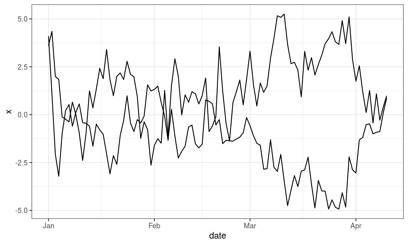
We can simulate cointegrated series assuming that \(\varepsilon_t\) in
\[ \Delta Y_t = \beta_0 + \beta_1 \Delta Y_{t-1} + \beta_2 Y_{t-1} + \varepsilon_t \]
is multivariate normal distributed.
##           [,1]    [,2]     [,3]
##   [1,] -1.0196 -0.6142  -0.7961
##   [2,]  1.7276  0.9038  -0.1201
##   [3,]  1.7463  0.4977  -0.7174
##   [4,]  1.1263  0.5162  -0.7929
##   [5,]  1.8858  1.6565   1.4163
##   [6,]  1.9840 -0.8705  -0.1100
##   [7,]  0.8058 -1.6116  -0.5430
##   [8,]  2.5154 -1.1793  -0.9609
##   [9,]  0.2421  0.1234  -1.7293
##  [10,]  0.8882 -1.4562  -1.3195
##  [11,]  2.4042 -0.3366  -0.4840
##  [12,]  0.6290 -1.0097  -0.2752
##  [13,]  0.9387 -1.6685  -1.1838
##  [14,]  1.1616 -1.8637   0.0625
##  [15,]  1.9550 -2.3363  -1.5793
##  [16,]  1.9627 -1.4635  -2.4213
##  [17,]  3.0953  0.0384  -1.4860
##  [18,]  0.3327  0.7472  -1.7295
##  [19,]  1.1418  0.1343  -1.0489
##  [20,]  1.6596  0.1665  -1.7719
##  [21,]  0.4693 -1.9359  -1.4337
##  [22,]  1.2669 -1.1636  -0.4412
##  [23,]  0.4397 -1.6052  -0.7097
##  [24,]  2.3267 -2.1257  -0.1934
##  [25,]  1.9344 -2.7140  -1.3804
##  [26,]  2.0031 -1.3368  -1.9743
##  [27,]  3.0365 -0.7465  -2.1452
##  [28,]  0.8378 -3.2959  -2.4943
##  [29,]  0.3035 -3.2189  -1.0372
##  [30,]  0.5171  1.0408  -0.2085
##  [31,] -1.5828 -0.0840  -0.9905
##  [32,] -0.3285  0.5088   0.3726
##  [33,] -1.4729  0.6808  -0.2077
##  [34,] -1.0198 -0.3316   0.7628
##  [35,]  0.6375 -0.6041   0.2880
##  [36,]  0.1427 -2.6870  -0.3048
##  [37,]  1.1872 -1.7402   1.0591
##  [38,]  0.2985 -1.9658   0.2734
##  [39,] -1.2566  0.4538   0.1288
##  [40,] -1.6232  1.8444  -1.2491
##  [41,] -2.3388  2.7166  -1.1473
##  [42,]  0.2906  3.5231  -1.1132
##  [43,] -0.5887  2.3137   0.5659
##  [44,] -1.5886  1.3747   0.5118
##  [45,] -1.4536  0.5599  -0.3090
##  [46,]  0.6876 -0.5673  -0.8293
##  [47,]  0.7272 -1.1505  -1.6571
##  [48,]  1.8788  1.4364  -0.8628
##  [49,] -0.0464  1.7740  -1.4978
##  [50,] -0.0972  2.7693  -0.4911
##  [51,] -0.6976  3.5211   0.2715
##  [52,]  0.1364  2.3161  -2.8410
##  [53,]  0.7187  3.2184  -2.0638
##  [54,]  0.7299  4.6659  -3.9833
##  [55,]  0.4152  4.4965  -4.2164
##  [56,]  0.4334  4.4785  -3.9072
##  [57,]  2.4025  4.4053  -3.9951
##  [58,]  3.2699  3.6282  -4.7302
##  [59,]  2.2951  4.9951  -5.6475
##  [60,]  2.8495  4.9621  -6.7682
##  [61,]  1.5350  5.6259  -7.2196
##  [62,]  1.9985  7.8426  -5.4048
##  [63,]  1.5342  6.1334  -6.1501
##  [64,] -0.7053  5.9287  -6.3934
##  [65,]  0.7267  5.2166  -7.2701
##  [66,]  2.9973  7.1754  -7.1197
##  [67,]  2.5625  8.6236  -8.5417
##  [68,]  1.5467  8.6546  -9.3575
##  [69,]  1.3024  8.7492  -7.8574
##  [70,]  0.0289  8.7403 -10.0260
##  [71,]  2.8516  8.3723  -9.3788
##  [72,]  3.7059  8.5971  -9.4111
##  [73,]  2.8584  7.5258 -10.1588
##  [74,]  3.6638  7.1051 -10.4496
##  [75,]  3.6859  5.1723 -10.0990
##  [76,]  4.7153  5.6631  -9.9829
##  [77,]  4.4710  5.8075 -10.8938
##  [78,]  6.1368  4.5939  -9.6848
##  [79,]  4.6093  4.7135 -12.0842
##  [80,]  5.1964  4.9847 -11.2377
##  [81,]  4.1206  5.0417 -10.0303
##  [82,]  4.8706  6.5303 -11.5173
##  [83,]  3.2075  7.1143 -11.2617
##  [84,]  3.7894  6.3483 -11.3592
##  [85,]  3.4247  7.2157 -10.3462
##  [86,]  4.6582  6.6338 -10.3494
##  [87,]  5.7347  5.6845 -12.5429
##  [88,]  7.0601  7.6796 -13.4185
##  [89,]  7.2606  8.0179 -13.3196
##  [90,]  6.9977  7.7841 -12.8841
##  [91,]  7.8181  7.3161 -13.1651
##  [92,]  7.2426  7.5070 -13.0424
##  [93,]  7.5951  7.7513 -12.7297
##  [94,]  7.5461  6.5649 -12.9936
##  [95,]  8.5196  7.5172 -13.2650
##  [96,]  8.1193  7.3621 -14.5875
##  [97,]  7.6551  6.2290 -15.8024
##  [98,]  7.5538  7.2694 -16.5240
##  [99,]  8.4789  8.2385 -15.1286
## [100,]  6.7067  6.7604 -15.5450
## [101,]  8.3683  7.5691 -11.5231
Testing time series properties
Unit root (ADF and KPSS) test
The ADF, available in the function adf.test() (in the package tseries) implements the t-test of \(H_0: \gamma = 0\) in the regression, below.
\[\begin{equation} \label{eqn:lagged-ts-regression} \Delta {{Y}_{t}}={{\beta }_{1}}+{{\beta }_{2}}t+\gamma {{Y}_{t-1}}+ \sum\limits_{i=1}^{m}{\delta_i \Delta {{Y}_{t-i}}+{{\varepsilon }_{t}}} \end{equation}\]
The null is therefore that series has a unit root. If only the series has a non-unit root, then it is stationary (rejection of null hypothesis).
The ADF test was parametrized with the alternative hypothesis of stationarity. This extends to following assumption in the model parameters;
\[ -2 \leq \gamma \leq 0\ \text{or } (-1 < 1+\phi < 1) \]
k in the function refers to the number of \(\delta\) lags, i.e., \(1, 2, 3, ...., m\) in the model equation.
The number of lags k defaults to trunc((length(x)-1)^(1/3)), where x is the series being tested. The default value of k corresponds to the suggested upper bound on the rate at which the number of lags, k, should be made to grow with the sample size for the general ARMA(p,q) setup citation(package = "tseries").
For a Dickey-Fueller test, only up to AR(1) time dependency in our stationary process is considered, we set k = 0. Hence we have no \(\delta\)s (lags) in our test.
The DF model can be written as:
\[ Y_t = \beta_1 + \beta_2 t + \phi Y_{t-1} + \varepsilon_t \]
It can be re-written so we can do a linear regression of \(\Delta Y_t\) against \(t\) and \(Y_{t-1}\) and test if \(\phi\) is different from 0. If only, \(\phi\) is not zero and assumption above (\(-1 < 1+\phi < 1\)) holds, the process is stationary. If \(\phi\) is straight up 0, then we have a random walk process – all white noise.
\[ \Delta {Y}_{t}=\beta_1+\beta_2 t+\gamma {Y}_{t-1} + \varepsilon_{t} \]
Alternative to above discussed tests, the Phillips-Perron test with its nonparametric correction for autocorrelation (essentially employing a HAC estimate of the long-run variance in a Dickey-Fuller-type test instead of parametric decorrelation) may be used. It is available in the function pp.test().
Unit root test based lag order differencing determination
An alternative to decomposition for removing trends is differencing [@woodward2017applied]. We define the order \(d\) difference operator as,
\[\begin{equation} \nabla^d x_t = (1-\mathbf{B})^d x_t, \label{eqn:order-d-difference-operator} \end{equation}\]
Where \(\mathbf{B}\) is the backshift operator (i.e., \(\mathbf{B}^k x_t = x_{t-k}\) for \(k \geq 1\)).
Applying the difference to a random walk, the most simple and widely used time series model, will yield a time series of Gaussian white noise errors \(\{w_t\}\):
\[\begin{equation} \begin{aligned} \nabla (x_t &= x_{t-1} + w_t) \\ x_t - x_{t-1} &= x_{t-1} - x_{t-1} + w_t \\ x_t - x_{t-1} &= w_t \end{aligned} \label{eqn:random-walk-series} \end{equation}\]
Unit testing: ADF
Vector autoregressive model (VAR)
VAR is a system regression model, i.e., there are more than one dependent variable. The regression is defined by a set of linear dynamic equations where each variable is specified as a function of an equal number of lags of itself and all other variables in the system. Any additional variable, adds to the modeling complexity by increasing an extra equation to be estimated.
The vector autoregression (VAR) model extends the idea of univariate autoregression to \(k\) time series regressions, where the lagged values of all \(k\) series appear as regressors. Put differently, in a VAR model we regress a vector of time series variables on lagged vectors of these variables. As for \(AR(p)\) models, the lag order is denoted by \(p\) so the \(VAR(p)\) model of two variables \(X_t\) and \(Y_t\) (\(k=2\)) is given by a vector of equations (Equation ??).
\[\begin{equation} \label{eqn:vector-regression-ts} \begin{split} \begin{aligned} Y_t =& \, \beta_{10} + \beta_{11} Y_{t-1} + \dots + \beta_{1p} Y_{t-p} + \gamma_{11} X_{t-1} + \dots + \gamma_{1p} X_{t-p} + u_{1t}, \\ X_t =& \, \beta_{20} + \beta_{21} Y_{t-1} + \dots + \beta_{2p} Y_{t-p} + \gamma_{21} X_{t-1} + \dots + \gamma_{2p} X_{t-p} + u_{2t}. \end{aligned} \end{split} \end{equation}\]
The \(\beta\)s and \(\gamma\)s can be estimated using OLS on each equation.
Simplifying this to a bivariate \(VAR(1)\), we can write the model in matrix form as:
\[\begin{equation} \label{eqn:matix-var1-model} Y_t = \beta_0 + \beta_1 Y_{t-1} + \mu_t \end{equation}\]
Where,
- \(Y_t, Y_{t-1}\) and \(\mu_t\) are (2 x 1) column vectors
- \(\beta_0\) is a (2 x 1) column vector
- \(\beta_1\) is a (2 x 2) matrix
also,
\[ Y_t = \begin{pmatrix} y_{1t} \\ y_{2t} \end{pmatrix},\ Y_{t-1} = \begin{pmatrix} y_{1t-1} \\ y_{2t-1} \end{pmatrix} \]
\[ \mu_t = \begin{pmatrix} \mu_{1t} \\ \mu_{2t} \end{pmatrix}, \beta_{0} = \begin{pmatrix} \beta_{10} \\ \beta_{20} \end{pmatrix}, \beta_{1} = \begin{pmatrix} \beta_{11} & \alpha_{11} \\ \alpha_{21} & \beta_{21} \end{pmatrix} \]
It is straightforward to estimate VAR models in R. A feasible approach is to simply use lm() for estimation of the individual equations. Furthermore, the vars package provides standard tools for estimation, diagnostic testing and prediction using this type of models.
Only when the assumptions presented below hold, the OLS estimators of the VAR coefficients are consistent and jointly normal in large samples so that the usual inferential methods such as confidence intervals and \(t\)-statistics can be used [@metcalfe2009introductory].
Two series \(w_{x,t}\) and \(w_{y,t}\) are bivariate white noise if they are stationary and their cross-covariances \(\gamma_{xy}(k) = Cov(w_{x,t}, w_{y, t+k})\) satisfies
\[ \gamma_{xx}(k) = \gamma_{yy}(k) = \gamma_{xy}(k) = 0\ \text{for all } k \neq 0 \]
The parameters of a var(p) model can be estimated using the ar function in R, which selects a best-fitting order \(p\) based on the smallest information criterion values.
##       [,1]  [,2]
## [1,] 1.009 0.782
## [2,] 0.782 0.947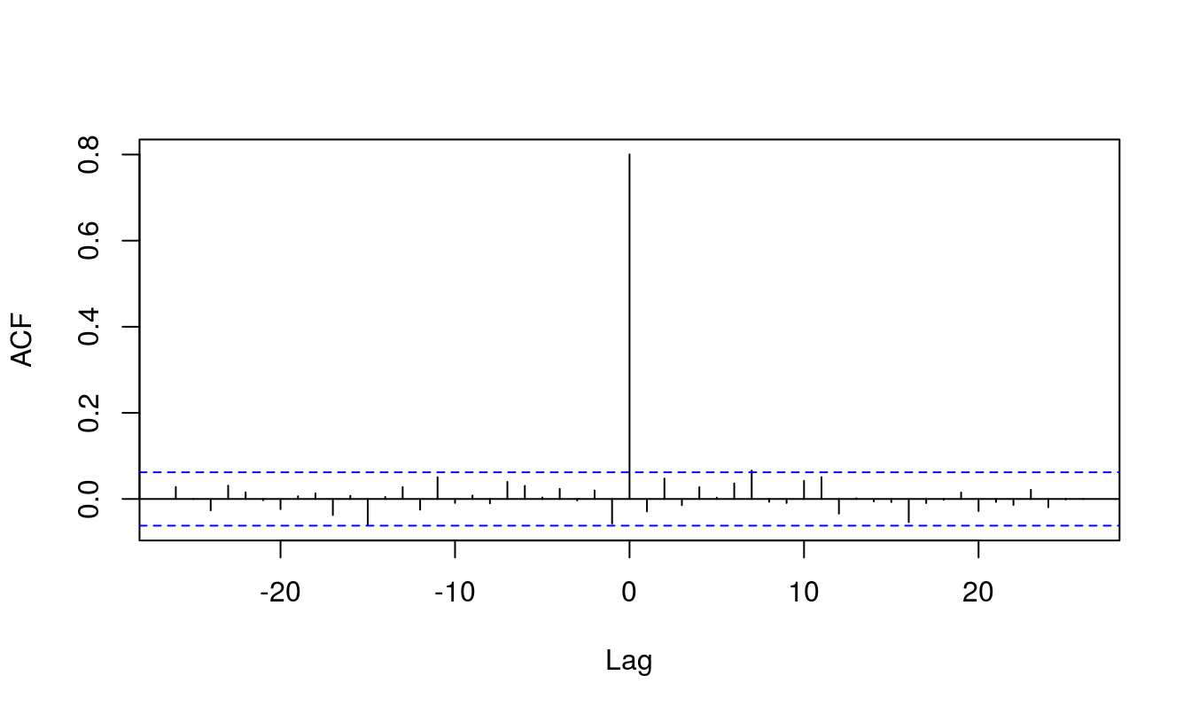
##      [,1] [,2]
## [1,]  0.4  0.3
## [2,]  0.2  0.1
## [1] 1.86 26.86## x y
## x 0.399 0.2813
## y 0.218 0.0419The structure of VARs also allows to jointly test restrictions across multiple equations. For instance, it may be of interest to test whether the coefficients on all regressors of the lag \(p\) are zero. This corresponds to testing the null that the lag order \(p-1\) is correct. Large sample joint normality of the coefficient estimates is convenient because it implies that we may simply use an \(F\)-test for this testing problem. The explicit formula for such a test statistic is rather complicated but fortunately such computations are easily done using the ttcode("R") functions we work with in this chapter. Just as in the case of a single equation, for a multiple equation model we choose the specification which has the smallest \(BIC(p)\), where
\[ \begin{aligned} BIC(p) =& \, \log\left[\text{det}(\widehat{\Sigma}_u)\right] + k(kp+1) \frac{\log(T)}{T}. \end{aligned} \]
with \(\widehat{\Sigma}_u\) denoting the estimate of the \(k \times k\) covariance matrix of the VAR errors and \(\text{det}(\cdot)\) denotes the determinant.
As for univariate distributed lag models, one should think carefully about variables to include in a VAR, as adding unrelated variables reduces the forecast accuracy by increasing the estimation error. This is particularly important because the number of parameters to be estimated grows qudratically to the number of variables modeled by the VAR.
Residual based cointegration test
Since the food commodities are spatially linked, more of so because they occupy the same domestic market, it is obvious that factor affecting price of one inevitably affects other, especially that of same crop in a nearby market. Having evidence for nonstationarity, it is of interest to test for a common nonstationary component by means of a cointegration test (Non-stationarity is more valid for development regionwise price series).
A two step method proposed by @hylleberg1990seasonal can be used to test for cointegration. The procedure simply regressess one series on the other and performs a unit root test on the residuals. This test is often named after @phillips1990asymptotic. Specifically, po.test() performs a Phillips-Perron test using an auxiliary regression without a constant and linear trend and the Newey-West estimator for the required long-run variance.
The test computes the Phillips-Ouliaris test for the null hypothesis that series is not cointegrated [@R-tseries].
Note po.test does not handle missing values, so we fix them through imputation. It is implemented through tidyr::fill(..., .direction = "down").
The problem with this approach is that it treats both series in an asymmetric fashion, while the concept of cointegration demands that the treatment be symmetric.
The po.test() function is testing the cointegration with Phillip’s Z_alpha test, which is the second residual-based test described by @phillips1990asymptotic. Because the po.test() will use the series at the first position to derive the residual used in the test, results would be determined by the series on the most left-hand side1.
The Phillips-Ouliaris test implemented in the ca.po() function from the urca package is different. In the ca.po() function, there are two cointegration tests implemented, namely “Pu” and “Pz” tests. Although both the ca.po() function and the po.test() function are supposed to do the Phillips-Ouliaris test,outcomes from both functions are completely different.
Similar to Phillip’s Z_alpha test, the Pu test also is not invariant to the position of each series and therefore would give different outcomes based upon the series on the most left-hand side. On the contrary, the multivariate trace statistic of Pz test has its appeal in that the outcome won’t change by the position of each series.
VAR based cointegration test
The standard tests proceeding in a symmetric manner stem from Johansen’s full-information maximum likelihood approach [@johansen1991estimation]. A general vector autoregressive model is similar to the AR(p) model except that each quantity is vector valued and matrices are used as the coefficients. The general form of the VAR(p) model, without drift, is given by:
\[\begin{equation} \label{eqn:var-general} {\bf y_t} = {\bf \mu} + A_1 {\bf y_{t-1}} + \ldots + A_j {\bf y_{t-j}} + {\bf \varepsilon_t} \end{equation}\]
Where \({\bf \mu}\) is the vector-valued mean of the series, \(A_i\) are the coefficient matrices for each lag and \({\bf \varepsilon_t}\) is a multivariate Gaussian noise term with mean zero.
At this stage we can form a Vector Error Correction Model (VECM) by differencing the series (Equation ??).
\[\begin{equation} \label{eqn:vecm-differenced} \Delta {\bf y_t} = {\bf \mu} + A {\bf y_{t-1}} + \Gamma_1 \Delta {\bf y_{t-1}} + \ldots + \Gamma_j \Delta {\bf y_{t-j}} + {\bf \varepsilon_t} \end{equation}\]
Where \(\Delta {\bf y_t} = {\bf y_t} - {\bf y_{t-1}}\) is the differencing operator, \(A\) is the coefficient matrix for the first lag and \(\Gamma_i\) are the matrices for each differenced lag.
For a \(p^{th}\) -order cointegrated vector autoregressive (VAR) model, the error correction form is (omitting deterministic components; both no intercept or trend in either cointegrating equation or test var), we may rewrite the VAR in the form of Equation ?? [@johansen1991estimation].
For more information refer to: - Eviews documentation - Quantstart post - Kevin kotze’s post
\[\begin{equation} \label{eqn:johansens} \Delta y_t = \Pi y_{t-1} + \sum_{j = 1}^{p-1} {\Gamma_j \Delta y_{t-j}} + \varepsilon_t \end{equation}\]
Where,
\[ \Pi = \sum^{p}_{i = 1}{A_{i}-I}; \Gamma = -\sum^{p}_{j = i + 1}{j} \]
(Although, for simplicity sake, we assume absence of deterministic trends, there are five popular scenarios of including such trends in a cointegration test. All of these are described in [@johansen1995identifying].)
Granger’s representation theorem asserts that if the coefficient matrix \(\Pi\) has reduced rank \(r < k\), then there exist \(kxr\) matrices \(\alpha\) and \(\beta\) each with rank \(k\) such that \(\Pi = \alpha \beta^{\prime}\) and \(\beta^{\prime}y_t\) is \(I(0)\).
To achieve this an eigenvalue decomposition of \(A\) is carried out. The rank of the matrix \(A\) is given by \(r\) and the Johansen test sequentially tests whether this rank \(r\) is equal to zero, equal to one, through to \(r=n-1\), where \(n\) is the number of time series under test.
The null hypothesis of \(r=0\) means that there is no cointegration at all. A rank \(r > 0\) implies a cointegrating relationship between two or possibly more time series.
The eigenvalue decomposition results in a set of eigenvectors. The components of the largest eigenvector admits the important property of forming the coefficients of a linear combination of time series to produce a stationary portfolio. Notice how this differs from the CADF test (often known as the Engle-Granger procedure) where it is necessary to ascertain the linear combination a priori via linear regression and ordinary least squares (OLS).
In summary, the test checks for the situation of no cointegration, which occurs when the matrix \(A=0\). So, starting with the base value of \(r\) (i.e., \(r=0\)), if the test statistic is greater than critical values of at the 10%, 5% and 1% levels, this would imply that we are able to reject the null of no cointegration. For the case r<=1, we if the calculated test statistic is below the critical values of, we are unable to reject the null, and the number of cointegrating vectors is between 0 and 1. The relevant tests are available in the function urca::ca.jo(). The basic version considers the eigenvalues of the matrix \(\Pi\) in the preceding equation.
Causality test
Causality test is VAR based approach to explain cause-effect relationship among endogenous variables. However, the Granger-causality [@granger1988causality] inference does not, of course, establish the real causation phenomena. If one of the variables is sufficiently correlated to the other so that forecast of former depends on the later to a considerable extent, then the first variable is granger-caused by the second one.
The Granger causality has been briefed to be useable test in certain cases of two series violating the stationarity assumption2.
@papana2014identifying state that GC test can only to applied if both the series are stationary3. Same paper also cautioned that VAR(1) models of cointegrated endogenous series will fail to capture long-run relationships. Therefore, the authors suggest surplus lag Granger-causality test be used if the series are a nonstationary data.
Common statistical tests and econometric models are interpreted based on cut-off probability value 5%. Where model selection is desired, model terms minimizing Akaike or Bayesian Information Criterion, or where relevant both, were selected.
VECM mathematical explanation
\[ \bf{X}_t = \bf{\Pi}_1 \bf{X}_{t-1} +...+ \bf{\Pi}_k \bf{X}_{t-k} + \bf{\mu} + \bf{\Phi D}_t + \bf{\varepsilon}_t , \quad (t = 1, ... , T), \]
the following two specifications of a VECM exist:
\[ \Delta \bf{X}_t = \bf{\Gamma}_1 \Delta \bf{X}_{t-1} + ... + \bf{\Gamma}_{k-1} \Delta \bf{X}_{t-k+1} + \bf{\Pi X}_{t-k} + \bf{\mu} + \bf{\Phi D}_t + \bf{\varepsilon}_t \]
where
\[ \bf{\Gamma}_i = - (\bf{I} - \bf{\Pi}_1 - ... - \bf{\Pi}_i), \quad (i = 1,..., k-1), \]
and
\[ \bf{\Pi} = -(\bf{I} - \bf{\Pi}_1 -...- \bf{\Pi}_k) \]
Notes: Loading matrix is the adjustment matrix (\(\alpha\) matrix). The elements of α determine the speed of adjustment to the long-run equilibrium.
The \(\bf{\Gamma}_i\) matrices contain the cumulative long-run impacts, hence if spec=“longrun” is choosen, the above VECM is estimated.
The other VECM specification is of the form:
\[ \Delta \bf{X}_t = \bf{\Gamma}_1 \Delta \bf{X}_{t-1} +...+ \bf{\Gamma}_{k-1} \Delta \bf{X}_{t-k+1} + \bf{\Pi X}_{t-1} + \bf{\mu} + \bf{\Phi D}_t + \bf{\varepsilon}_t \]
where
\[\bf{\Gamma}_i = - (\bf{\Pi}_{i+1} +...+ \bf{\Pi}_k), \quad(i = 1,..., k-1)\],
and
\[\bf{\Pi} = -(\bf{I} - \bf{\Pi}_1 -...- \bf{\Pi}_k)\].
The \(\bf{\Pi}\) matrix is the same as in the first specification. However, the \(\bf{\Gamma}_i\) matrices now differ, in the sense that they measure transitory effects, hence by setting spec=“transitory” the second VECM form is estimated. Please note that inferences drawn on \(\bf{\Pi}\) will be the same, regardless which specification is choosen and that the explanatory power is the same, too.
Some notes
In his blog post kevin kotze https://kevinkotze.github.io/ts-10-tut/ mentions fits error correction model with a linear regression. Therein for the gold and silver dataset, the regression residuals of gold ~ silver are verified for stationarity and only then inferred that they may be cointegrated.
How to detect order of integration ?
Checking for order of integration for a single variable involves first testing with Dickey Fueller. Initially we use all deterministic components one by one and use lag selection with probably “BIC”. For first order integrated series, we should observe that we cannot reject null hypothesis of no unit root. Thenafter we perform the same test with first order differenced value of the same variable. Thenafter, if we should find enough evidence of rejecting null hypothesis of DF-test, i.e., null: there exists unit root, we can conclude that the series is integrated of order 1.
interestingly, linear regression fit of dickey fueller test is pretty simple, and demonstrated below in. However, it has some petty differences in coefficient estimates, that may be because of the way differenced and lagged values are handled differently inside a dataframe and in a independent series. (Verify also that!)
An error correction model for the gold silver dataset is set with linear regression as follow: (Note some datapoints are eliminated to match the length of vector for analysis)
gold.d <- diff(gold)[-1]
silver.d <- diff(silver)[-1]
error.ecm1 <- gold.eq$residuals[-1:-2]
gold.d1 <- diff(gold)[-(length(gold) - 1)]
silver.d1 <- diff(silver[-(length(silver) - 1)])
The model specification is:
ecm.gold <- lm(gold.d ~ error.ecm1 + gold.d1 + silver.d1)
summary(ecm.gold)
The regression output is used to interpret infer about the \(\alpha\) (term error.ecm1). If the alpha (speed of adjustment) is insignificant and close to zero, the differenced series will be said to be be weakly exogenous with respect to the cointegrating parameters since it does not adjust to past deviation from long-run equilibrium. The long run regression is infact the simple first stage regression:
gold.eq <- lm(gold ~ silver, data = data)Same could be done for both silver and gold. With similar kind of error correction model specification with silver as dependent variable. Results can be drastically different for two series (as is for gold and silver). In the blog’s case, the alpha (speed of adj) is negative and significant, so silver does all the work to get the two variables back towards the equilibrium path. This implies that there is Granger causality from gold to silver and that it takes about 1/0.0078 (Estimate of error.ecm1) periods to regurn to equilibrium.
Bibliography
CRAN’s var package vignette is pretty explanatory. It delves in quickly into the intricacies of VAR and VECM modeling placing cointegration relationship at the center. https://cran.r-project.org/web/packages/vars/vignettes/vars.pdf
Analysis of integrated and cointegrated time series with R. url: https://link.springer.com/content/pdf/bfm%3A978-0-387-75967-8%2F1.pdf @book{pfaff2008analysis, title={Analysis of integrated and cointegrated time series with R}, author={Pfaff, Bernhard}, year={2008}, publisher={Springer Science & Business Media} }
Time series Chapter 6, Applied Econometrics with R url: https://eeecon.uibk.ac.at/~zeileis/teaching/AER/Ch-TimeSeries.pdf
Principles of Econometrics with R; Time series: non stationarity https://bookdown.org/ccolonescu/RPoE4/time-series-nonstationarity.html
Applied Econometrics, Econ 508 - Fall 2014, Professor: Roger Koenker, e-TA 8: Unit Roots and Cointegration
http://www.econ.uiuc.edu/~econ508/R/e-ta8_R.html
Note: This page has an embeded R script that has function called johansen() to carry out the test.
Johansen Test for Cointegrating Time Series Analysis in R https://www.quantstart.com/articles/Johansen-Test-for-Cointegrating-Time-Series-Analysis-in-R/
Tutorial: Cointegration, Kevin Kotze https://kevinkotze.github.io/ts-10-tut/
Introduction to econometrics with R, Cointegration https://www.econometrics-with-r.org/16-3-cointegration.html
@article{sims1990inference, title={Inference in linear time series models with some unit roots}, author={Sims, Christopher A and Stock, James H and Watson, Mark W}, journal={Econometrica: Journal of the Econometric Society}, pages={113–144}, year={1990}, publisher={JSTOR} }
Panel data econometrics in R, plm package. https://mran.microsoft.com/snapshot/2017-10-11/web/packages/plm/vignettes/plm.pdf