Time Series: Basic Analysis

Background

This post is the first in a series of upcoming blog that tries to describe application of a lesser used technique in econometrics – time series analysis. I make extensive use of datasets available in several R packages – mostly the tsibbledata package. Furthermore, an external package hosted in github.com/FinYang/tsdl repo will be used.

## [1] 12

## Time Series Data Library: 648 time series  
## 
##                        Frequency
## Subject                 0.1 0.25   1   4   5   6  12  13  52 365 Total
##   Agriculture             0    0  37   0   0   0   3   0   0   0    40
##   Chemistry               0    0   8   0   0   0   0   0   0   0     8
##   Computing               0    0   6   0   0   0   0   0   0   0     6
##   Crime                   0    0   1   0   0   0   2   1   0   0     4
##   Demography              1    0   9   2   0   0   3   0   0   2    17
##   Ecology                 0    0  23   0   0   0   0   0   0   0    23
##   Finance                 0    0  23   5   0   0  20   0   2   1    51
##   Health                  0    0   8   0   0   0   6   0   1   0    15
##   Hydrology               0    0  42   0   0   0  78   1   0   6   127
##   Industry                0    0   9   0   0   0   2   0   1   0    12
##   Labour market           0    0   3   4   0   0  17   0   0   0    24
##   Macroeconomic           0    0  18  33   0   0   5   0   0   0    56
##   Meteorology             0    0  18   0   0   0  17   0   0  12    47
##   Microeconomic           0    0  27   1   0   0   7   0   1   0    36
##   Miscellaneous           0    0   4   0   1   1   3   0   1   0    10
##   Physics                 0    0  12   0   0   0   4   0   0   0    16
##   Production              0    0   4  14   0   0  28   1   1   0    48
##   Sales                   0    0  10   3   0   0  24   0   9   0    46
##   Sport                   0    1   1   0   0   0   0   0   0   0     2
##   Transport and tourism   0    0   1   1   0   0  12   0   0   0    14
##   Tree-rings              0    0  34   0   0   0   1   0   0   0    35
##   Utilities               0    0   2   1   0   0   8   0   0   0    11
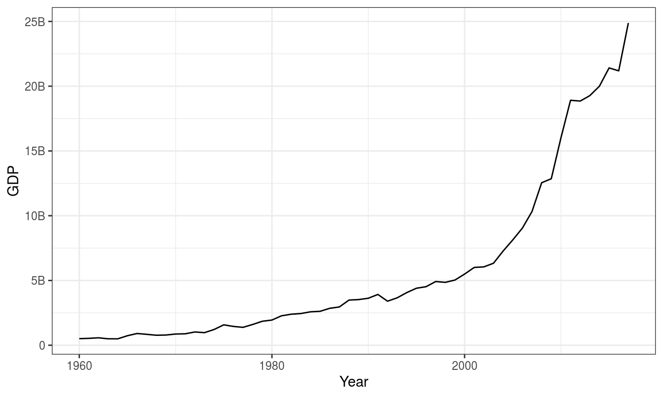
##   Total                   1    1 300  64   1   1 240   3  16  21   648

For starter, let’s take globaleconomy dataset in tsibbledata package. Let’s consider GDP values of Nepal as example. It should be noted that values are expressed in $USD (with conversion rate of February 2019).

There are several important considerations about this dataset. These could also be phrased as questions regarding properties of time series.

Questions regarding time series

• Is there a trend, meaning that, on average, the measurements tend to increase (or decrease) over time?
• Is there seasonality, meaning that there is a regularly repeating pattern of highs and lows related to calendar time such as seasons, quarters, months, days of the week, and so on?
• Are there outliers? In regression, outliers are far away from your line. With time series data, your outliers are far away from your other data.
• Is there a long-run cycle or period unrelated to seasonality factors?
• Is there constant variance over time, or is the variance non-constant?
• Are there any abrupt changes to either the level of the series or the variance?

Time series properties

A non trending data shows variation in values as if it were drawn from a random distribution. For instance,

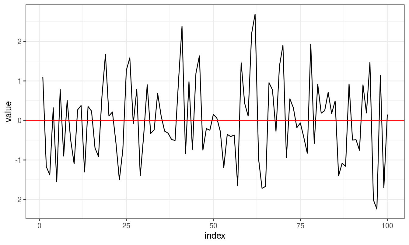
There is no consistent trend (upward or downward) over the entire time span. The series appears to slowly wander up and down. The horizontal line drawn at value = 0 indicates the mean of the series.

It’s difficult to judge whether the variance is constant or not.

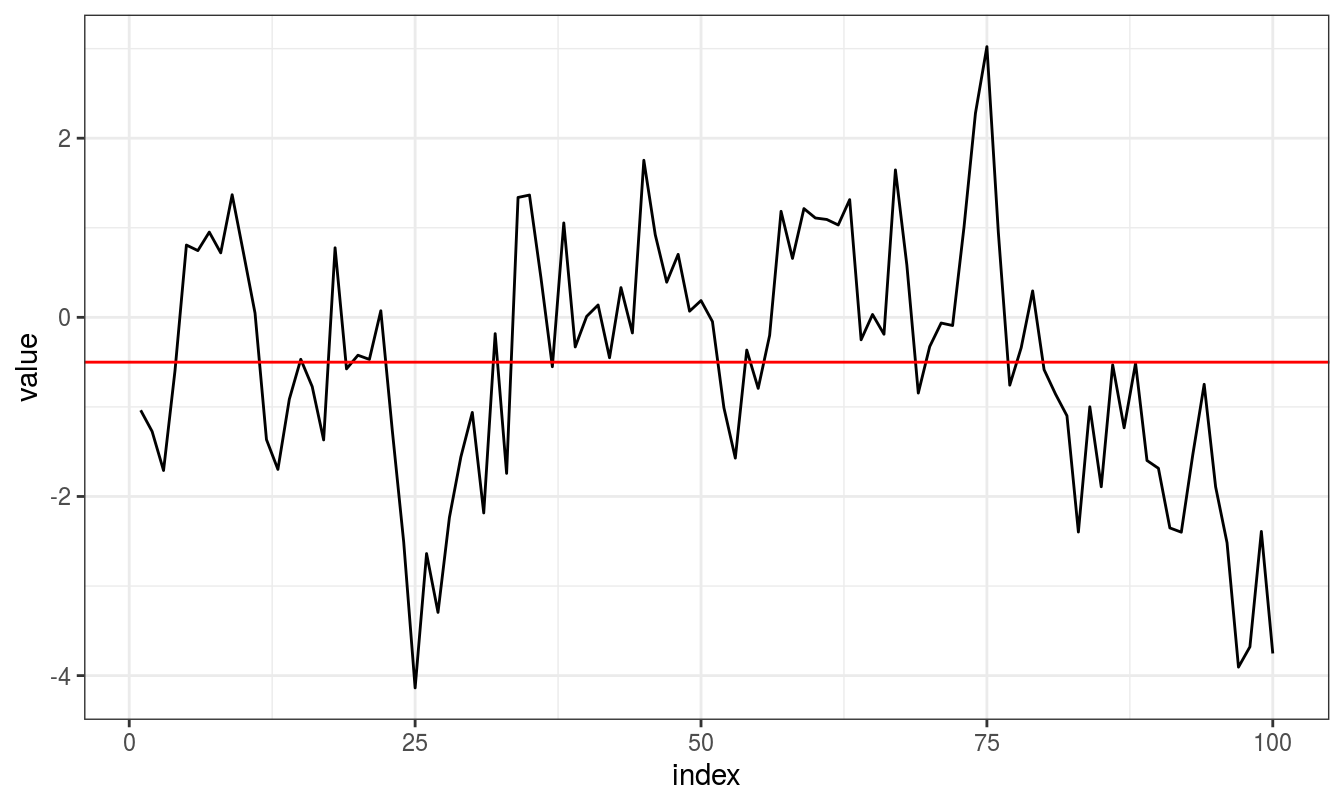
Notice that the series tends to stay on the same side of the mean (above or below) for a while and then wanders to the other side.

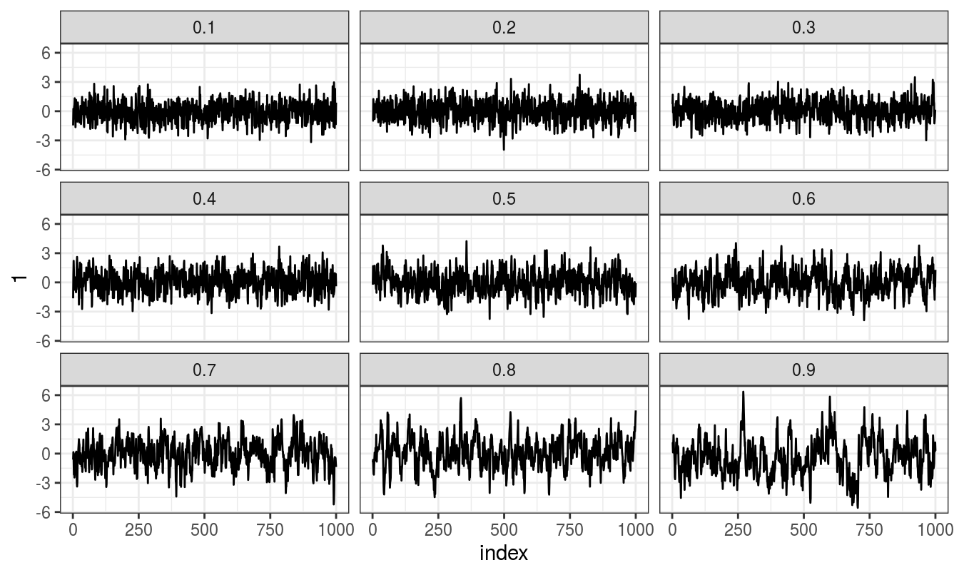
To conceptualize autoregressive model, we simulate multiple ARIMA(p,0,0) series of various autoregressive coefficients and then feed that into model for coefficient estimation. The acronym ARIMA stands for Auto-Regressive Integrated Moving Average. Lags of the stationarized series in the forecasting equation are called “autoregressive” terms, lags of the forecast errors are called “moving average” terms, and a time series which needs to be differenced to be made stationary is said to be an “integrated” version of a stationary series. Random-walk and random-trend models, autoregressive models, and exponential smoothing models are all special cases of ARIMA models^{[https://people.duke.edu/~rnau/411arim.htm#pdq]}[The page also has symbolism and model representations of popular ARIMA model].

A nonseasonal ARIMA model is classified as an “ARIMA(p,d,q)” model, where:

• p is the number of autoregressive terms,
• d is the number of nonseasonal differences needed for stationarity, and
• q is the number of lagged forecast errors in the prediction equation.

Some well defined variants of ARIMA models are:

• ARIMA(1,0,0) = first-order autoregressive model
• ARIMA(0,1,0) = random walk
• ARIMA(1,1,0) = differenced first-order autoregressive model
• ARIMA(0,1,1) without constant = simple exponential smoothing
• ARIMA(0,1,1) with constant = simple exponential smoothing with growth
• ARIMA(0,2,1) or (0,2,2) without constant = linear exponential smoothing
• ARIMA(1,1,2) with constant = damped-trend linear exponential smoothing

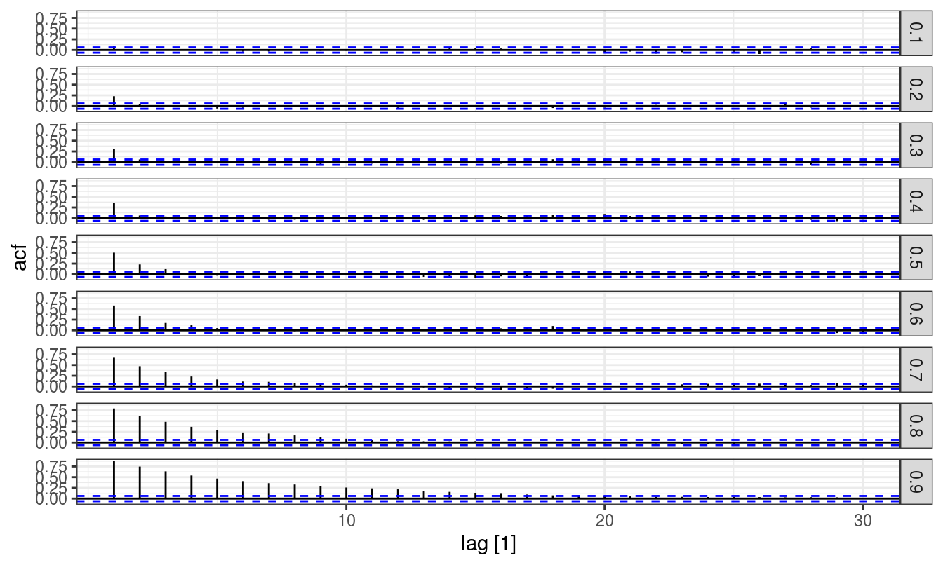
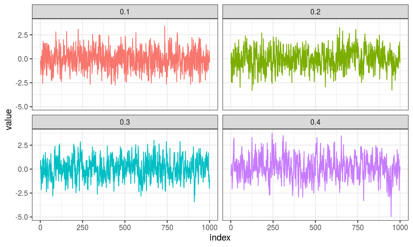
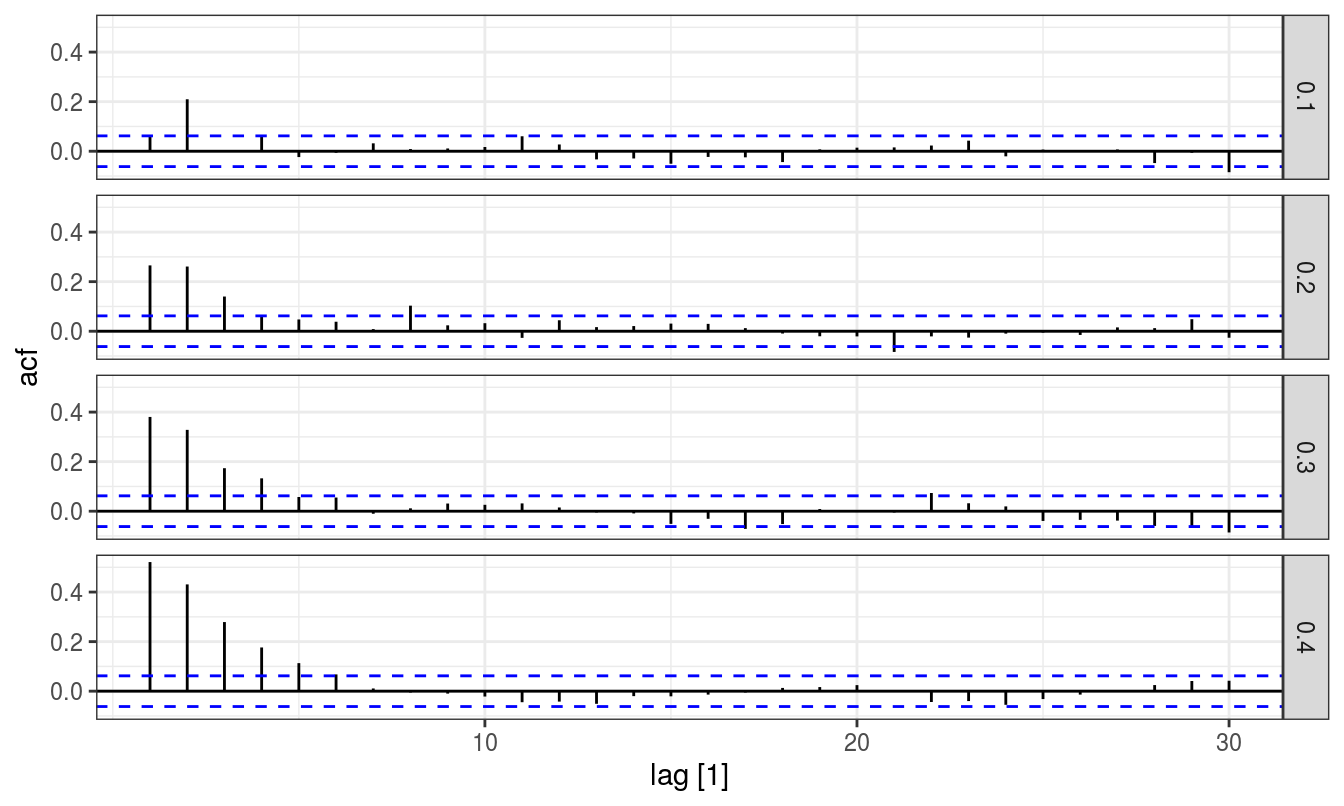
Firstly, for autoregressive coefficients (\(phi\)) of range 0.1 to 0.9, 20 simulation runs are made for \(p = 1\) autoregressive processes.

Here second order autoregressive model can be fitted similarly, arguably simulation runs are unnecessary when several time points are being considered.

For general working and modeling possibilities with arima, I refer reader to Hyndman’s blog post: https://otexts.com/fpp2/arima-r.html. The post details an algorithm for automatic arima model fitting.