Tidyverse and tidbits
- Ideas surrounding tidy evaluation
- quote() and eval()
- Why quote at-all
- Resolved messy data with tidy evaluation
- List behavior
- Using pmap to perform list operations inside a dataframe
- Apply a function to certain columns only, by rows
- Do any arbitrary operation
- Using dplyr functions inside your own functions
- Effiecient ways to operate on list
- Binds each element as row but third element is list
- Produces rowbinding for dataframe but doesn’t work with list elements
- Tibble and map data to list column in isolation
- Modeling, exploration, summary extraction and visualization examples using dplyr verbs.
- Workarounds on unequal length lists
- Quick saving dataframe as image/vector
Ideas surrounding tidy evaluation
R code is a tree
Every expression in R can be broken down to a form represented by a tree. For instance, on top of the tree there is “a function call” followed by it’s branches: first child = function name itself, other children = function arguments. Complex calls have multiple levels of branching.
The code tree could be captured by quoting
expr() quotes your(function developer) expression
f1 <- function(z) expr(z)
f1(a + b)
enexpr() quotes user’s expression
f2 <- function(z) enexpr(z)
f2(x + y)
Quoting and unquoting of expression enables building up of complex code trees
Unquoting is achieved by bang bang operator (!!)
For example, let’s create a function that makes scatter plot when fed a dataframe, x-variable and y-variable:
scatter_maker <- function(df, xvar, yvar) {
  xvar <- enexpr(xvar)
  yvar <- enexpr(yvar)

  ggplot(df, aes(!!xvar, !!yvar)) +
    geom_point()
}
The function is executed in the demo below:
scatter_maker(mtcars, disp, mpg) +
  theme_bw()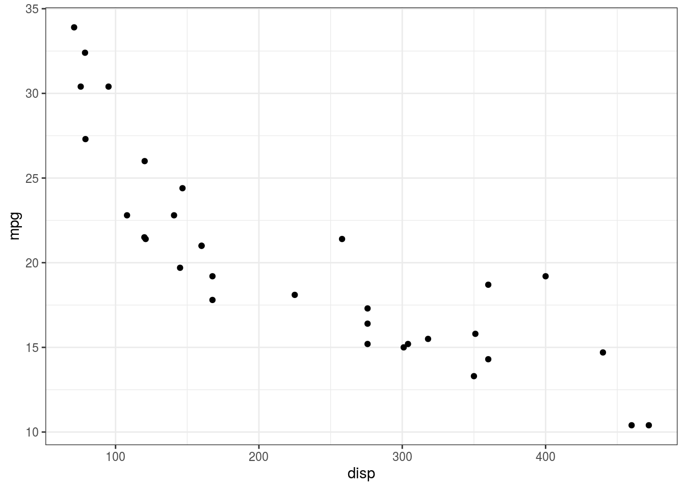
Figure 1: Scatterplot of displacement versus miles per gallon of mtcars dataset
- Quosures capture both expression and environment
quote() and eval()
- Quoting an expression is a bit like quoting a string
hm_quoted <- quote(height / mass)
hm_quoted
## height/mass- But it’s R code that can be evaluated and with a data mask it works!
# eval(hm_quoted) # doesn't work because lacks data mask
head(eval(hm_quoted, starwars)) # works
## [1] 2.233766 2.226667 3.000000 1.485294 3.061224 1.483333Why quote at-all
- Data masking
- Allows you to refer to data objects directly
# because transmute() is a quoting function,
transmute(starwars, height / mass)
## # A tibble: 87 x 1
## `height/mass`
## <dbl>
## 1 2.23
## 2 2.23
## 3 3
## 4 1.49
## 5 3.06
## 6 1.48
## 7 2.2
## 8 3.03
## 9 2.18
## 10 2.36
## # … with 77 more rows# # unlike below where data objects could not be directly refered to
# height / mass
# starwars$height / starwars$massResolved messy data with tidy evaluation
A messy dataset exists despite all the sufferings. No wonder, it is resolvable, though.
The identification is done through keywords like “gen1”, “gen2”, … The rowtype and the height columns occur in precedence to the identifier key. Our function will break apart the respective entries of rowtype and height into separate columns.
dat <- tibble(mess = c("row:Three-row", "ht:Short height", "gen1",
                       "row:Two-row", "ht:Tall height", "gen2",
                       "row:Three-row", "ht:Short height", "gen4",
                       "ht:Tall height", "row:Three-row", "gen3",
                       "row:Three-row"))

dat
## # A tibble: 13 x 1
## mess
## <chr>
## 1 row:Three-row
## 2 ht:Short height
## 3 gen1
## 4 row:Two-row
## 5 ht:Tall height
## 6 gen2
## 7 row:Three-row
## 8 ht:Short height
## 9 gen4
## 10 ht:Tall height
## 11 row:Three-row
## 12 gen3
## 13 row:Three-rowLet’s define new verb untangle2().
untangle2 <- function(df, regex, orig, new) {
  orig <- enexpr(orig)
  new <- sym(quo_name(enexpr(new)))
  # orig <- enquo(orig) # this too works!
  # new <- sym(quo_name(enquo(new))) # this too works!

  df %>%
    mutate(
      !!new := if_else(grepl(regex, !! orig), !! orig, NA_character_)
    ) %>%
    fill(!! new) %>%
    filter(! grepl(regex, !! orig))
}

dat %>%
  untangle2("^row", mess, rowtype) %>%
  untangle2("^ht", mess, height)
## # A tibble: 4 x 3
## mess rowtype height
## <chr> <chr> <chr>
## 1 gen1 row:Three-row ht:Short height
## 2 gen2 row:Two-row ht:Tall height
## 3 gen4 row:Three-row ht:Short height
## 4 gen3 row:Three-row ht:Tall heightList behavior
When supplied a list to a dataframe as argument, list elements will be attempted to be supplied as individual column vectors. As long as the length of list element is same as the number of rows in dataframe, columns will be appended without an error.
However, if the complete list object is to be added in as a column vector, it’s identity needs to be preserved. Function I() preserves the identity by wrapping the object around “AsIs” class. For example, let’s create a dataframe with a list object containing it’s elements.
# all list elements of equal length as `nrow`.
df1 <- data.frame(x = 1:3, y = list(3:5, 4:6, 5:7))
df
## function (x, df1, df2, ncp, log = FALSE)
## {
## if (missing(ncp))
## .Call(C_df, x, df1, df2, log)
## else .Call(C_dnf, x, df1, df2, ncp, log)
## }
## <bytecode: 0x942df38>
## <environment: namespace:stats># this results in error due to an attempt to bind list elements of unequal length as columns
# df <- data.frame(x = 1:3, y = list(3:9, 1:3, 1:3))When dealing with unequal length lists, try wrapping the list around in I() function, as shown below.
df <- data.frame(x = 1:3, y = I(list(3:9, 1:3, 1:3)))
df
## x y
## 1 1 3, 4, 5,....
## 2 2 1, 2, 3
## 3 3 1, 2, 3# Distinction can be made based on the classes
purrr::compose(class)(list(3:9, 1:3, 1:3))## [1] "list"purrr::compose(class, I)(list(3:9, 1:3, 1:3)) # compose applies multiple functions right to left## [1] "AsIs"Using pmap to perform list operations inside a dataframe
params <- expand.grid(param_a = c(2, 4, 6),
                      param_b = c(3, 6, 9),
                      param_c = c(50, 100),
                      param_d = c(1, 0))

params %>%
  knitr::kable(caption = "Fictious data set to be used as template",
               format = "html") %>%
kableExtra::kable_styling(bootstrap_options = "striped", font_size = 10)| param_a | param_b | param_c | param_d |
|---|---|---|---|
| 2 | 3 | 50 | 1 |
| 4 | 3 | 50 | 1 |
| 6 | 3 | 50 | 1 |
| 2 | 6 | 50 | 1 |
| 4 | 6 | 50 | 1 |
| 6 | 6 | 50 | 1 |
| 2 | 9 | 50 | 1 |
| 4 | 9 | 50 | 1 |
| 6 | 9 | 50 | 1 |
| 2 | 3 | 100 | 1 |
| 4 | 3 | 100 | 1 |
| 6 | 3 | 100 | 1 |
| 2 | 6 | 100 | 1 |
| 4 | 6 | 100 | 1 |
| 6 | 6 | 100 | 1 |
| 2 | 9 | 100 | 1 |
| 4 | 9 | 100 | 1 |
| 6 | 9 | 100 | 1 |
| 2 | 3 | 50 | 0 |
| 4 | 3 | 50 | 0 |
| 6 | 3 | 50 | 0 |
| 2 | 6 | 50 | 0 |
| 4 | 6 | 50 | 0 |
| 6 | 6 | 50 | 0 |
| 2 | 9 | 50 | 0 |
| 4 | 9 | 50 | 0 |
| 6 | 9 | 50 | 0 |
| 2 | 3 | 100 | 0 |
| 4 | 3 | 100 | 0 |
| 6 | 3 | 100 | 0 |
| 2 | 6 | 100 | 0 |
| 4 | 6 | 100 | 0 |
| 6 | 6 | 100 | 0 |
| 2 | 9 | 100 | 0 |
| 4 | 9 | 100 | 0 |
| 6 | 9 | 100 | 0 |
# using map function to obtain a list
df.preprocessed <- as.tbl(params) %>%
  mutate(test_var = purrr::map(param_a, function(x){rep(5, x)}))

# using pmap for more flexible operation and unnesting to get expanded list
df.preprocessed1 <- dplyr::as.tbl(params) %>%
  mutate(test_var = purrr::pmap(.,
                                function(param_a, param_b, ...){
                                  rep(5, param_a) * param_b
                                })) %>%
  tidyr::unnest()
## Warning: `cols` is now required.
## Please use `cols = c(test_var)`# rowwise operation will also enable the same
my_fun <- function(param_a, param_b){
rep(5, param_a) * param_b
}
dplyr::as.tbl(params) %>%
rowwise() %>%
dplyr::mutate(test_var = list(my_fun(param_a, param_b))) %>%
tidyr::unnest()## Warning: `cols` is now required.
## Please use `cols = c(test_var)`## # A tibble: 144 x 5
## param_a param_b param_c param_d test_var
## <dbl> <dbl> <dbl> <dbl> <dbl>
## 1 2 3 50 1 15
## 2 2 3 50 1 15
## 3 4 3 50 1 15
## 4 4 3 50 1 15
## 5 4 3 50 1 15
## 6 4 3 50 1 15
## 7 6 3 50 1 15
## 8 6 3 50 1 15
## 9 6 3 50 1 15
## 10 6 3 50 1 15
## # … with 134 more rows# of all pmap solution could be the most flexible option
dplyr::as.tbl(params) %>%
dplyr::mutate(test_var = purrr::pmap(list(x = param_a
,y = param_b
,z = param_c
,u = param_d),
~ rep(5,..1)*..2)
)## # A tibble: 36 x 5
## param_a param_b param_c param_d test_var
## <dbl> <dbl> <dbl> <dbl> <list>
## 1 2 3 50 1 <dbl [2]>
## 2 4 3 50 1 <dbl [4]>
## 3 6 3 50 1 <dbl [6]>
## 4 2 6 50 1 <dbl [2]>
## 5 4 6 50 1 <dbl [4]>
## 6 6 6 50 1 <dbl [6]>
## 7 2 9 50 1 <dbl [2]>
## 8 4 9 50 1 <dbl [4]>
## 9 6 9 50 1 <dbl [6]>
## 10 2 3 100 1 <dbl [2]>
## # … with 26 more rowsApply a function to certain columns only, by rows
mtcars %>%
  select(am, gear, carb) %>%
  purrrlyr::by_row(sum, .collate = "cols", .to = "sum_am_gear_carb")
## # A tibble: 32 x 4
## am gear carb sum_am_gear_carb
## <dbl> <dbl> <dbl> <dbl>
## 1 1 4 4 9
## 2 1 4 4 9
## 3 1 4 1 6
## 4 0 3 1 4
## 5 0 3 2 5
## 6 0 3 1 4
## 7 0 3 4 7
## 8 0 4 2 6
## 9 0 4 2 6
## 10 0 4 4 8
## # … with 22 more rowsDo any arbitrary operation
mtcars %>%
  group_by(cyl) %>%
  do(models = lm(mpg ~ drat + wt, data = .)) %>%
  broom::tidy(models)
## # A tibble: 9 x 6
## # Groups: cyl [3]
## cyl term estimate std.error statistic p.value
## <dbl> <chr> <dbl> <dbl> <dbl> <dbl>
## 1 4 (Intercept) 33.2 17.1 1.94 0.0877
## 2 4 drat 1.32 3.45 0.384 0.711
## 3 4 wt -5.24 2.22 -2.37 0.0456
## 4 6 (Intercept) 30.7 7.51 4.08 0.0151
## 5 6 drat -0.444 1.17 -0.378 0.725
## 6 6 wt -2.99 1.57 -1.91 0.129
## 7 8 (Intercept) 29.7 7.09 4.18 0.00153
## 8 8 drat -1.47 1.63 -0.903 0.386
## 9 8 wt -2.45 0.799 -3.07 0.0107The do call is combined with group_by to get any summary of current dataframe
iris %>%
  group_by(Species) %>%
  do({
    mod <- lm(Sepal.Length ~ Sepal.Width, data = .)
    pred <- predict(mod, newdata = .["Sepal.Width"])
    data.frame(., pred)
  })
## # A tibble: 150 x 6
## # Groups: Species [3]
## Sepal.Length Sepal.Width Petal.Length Petal.Width Species pred
## <dbl> <dbl> <dbl> <dbl> <fct> <dbl>
## 1 5.1 3.5 1.4 0.2 setosa 5.06
## 2 4.9 3 1.4 0.2 setosa 4.71
## 3 4.7 3.2 1.3 0.2 setosa 4.85
## 4 4.6 3.1 1.5 0.2 setosa 4.78
## 5 5 3.6 1.4 0.2 setosa 5.12
## 6 5.4 3.9 1.7 0.4 setosa 5.33
## 7 4.6 3.4 1.4 0.3 setosa 4.99
## 8 5 3.4 1.5 0.2 setosa 4.99
## 9 4.4 2.9 1.4 0.2 setosa 4.64
## 10 4.9 3.1 1.5 0.1 setosa 4.78
## # … with 140 more rows# # same thing could be done through explicit function call with do
# iris %>%
# group_by(Species) %>%
# do((function(df) {
# mod <- lm(Sepal.Length ~ Sepal.Width, data = df)
# pred <- predict(mod,newdata = df["Sepal.Width"])
# data.frame(df,pred)
# })(.))Using dplyr functions inside your own functions
Create column selection/extraction function, for example.
extract_vars <- function(data, some_string){
  data %>%
    select_(lazyeval::interp(~contains(some_string))) -> data

  return(data)
}

extract_vars(mtcars, "drat")
## Warning: select_() is deprecated.
## Please use select() instead
##
## The 'programming' vignette or the tidyeval book can help you
## to program with select() : https://tidyeval.tidyverse.org
## This warning is displayed once per session.## drat
## Mazda RX4 3.90
## Mazda RX4 Wag 3.90
## Datsun 710 3.85
## Hornet 4 Drive 3.08
## Hornet Sportabout 3.15
## Valiant 2.76
## Duster 360 3.21
## Merc 240D 3.69
## Merc 230 3.92
## Merc 280 3.92
## Merc 280C 3.92
## Merc 450SE 3.07
## Merc 450SL 3.07
## Merc 450SLC 3.07
## Cadillac Fleetwood 2.93
## Lincoln Continental 3.00
## Chrysler Imperial 3.23
## Fiat 128 4.08
## Honda Civic 4.93
## Toyota Corolla 4.22
## Toyota Corona 3.70
## Dodge Challenger 2.76
## AMC Javelin 3.15
## Camaro Z28 3.73
## Pontiac Firebird 3.08
## Fiat X1-9 4.08
## Porsche 914-2 4.43
## Lotus Europa 3.77
## Ford Pantera L 4.22
## Ferrari Dino 3.62
## Maserati Bora 3.54
## Volvo 142E 4.11Effiecient ways to operate on list
x <- list(
  list(name = "sue", number = 1, veg = c("onion", "carrot")),
  list(name = "doug", number = 2, veg = c("potato", "beet"))
)
Base rbind() returns a matrix of lists. However, a complete list object x is packed in a single row, with two list columns for each next level list.
rbind(x)## [,1] [,2]
## x List,3 List,3Binds each element as row but third element is list
Throwing a do.call() call leads to desired results.
do.call(rbind, x)## name number veg
## [1,] "sue" 1 Character,2
## [2,] "doug" 2 Character,2do.call(rbind, x) %>% class()## [1] "matrix"Produces rowbinding for dataframe but doesn’t work with list elements
map_dfr(x, ~ .x[c("name", "number")])## # A tibble: 2 x 2
## name number
## <chr> <dbl>
## 1 sue 1
## 2 doug 2Tibble and map data to list column in isolation
tibble(
  name = map_chr(x, "name"),
  number = map_dbl(x, "number"),
  veg = map(x, "veg")
)
## # A tibble: 2 x 3
## name number veg
## <chr> <dbl> <list>
## 1 sue 1 <chr [2]>
## 2 doug 2 <chr [2]>Modeling, exploration, summary extraction and visualization examples using dplyr verbs.
gap <- gapminder %>%
  filter(continent == "Asia") %>%
  mutate(yr1952 = year - 1952)

ggplot(gap, aes(x = lifeExp, y = country)) +
  geom_point()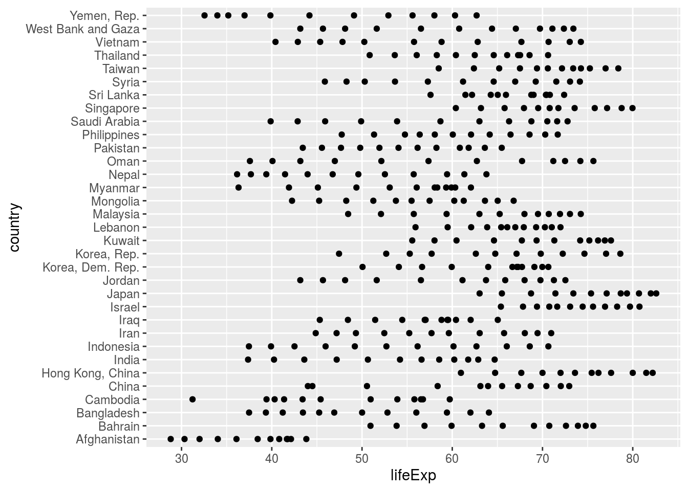
gap <- gap %>%
  mutate(country = fct_reorder2(country, .x = year, .y = lifeExp))

ggplot(gap, aes(x = lifeExp, y = country)) +
  geom_point()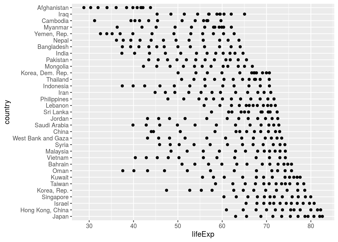
gap_nested <- gap %>%
  group_by(country) %>%
  nest()

gap_nested$data[[3]]
## # A tibble: 12 x 6
## continent year lifeExp pop gdpPercap yr1952
## <fct> <int> <dbl> <int> <dbl> <dbl>
## 1 Asia 1952 37.5 46886859 684. 0
## 2 Asia 1957 39.3 51365468 662. 5
## 3 Asia 1962 41.2 56839289 686. 10
## 4 Asia 1967 43.5 62821884 721. 15
## 5 Asia 1972 45.3 70759295 630. 20
## 6 Asia 1977 46.9 80428306 660. 25
## 7 Asia 1982 50.0 93074406 677. 30
## 8 Asia 1987 52.8 103764241 752. 35
## 9 Asia 1992 56.0 113704579 838. 40
## 10 Asia 1997 59.4 123315288 973. 45
## 11 Asia 2002 62.0 135656790 1136. 50
## 12 Asia 2007 64.1 150448339 1391. 55gap_fitted <- gap_nested %>%
mutate(fit = map(data, ~ lm(lifeExp ~ yr1952, data = .x)))
gap_fitted## # A tibble: 33 x 3
## # Groups: country [142]
## country data fit
## <fct> <list> <list>
## 1 Afghanistan <tibble [12 × 6]> <lm>
## 2 Bahrain <tibble [12 × 6]> <lm>
## 3 Bangladesh <tibble [12 × 6]> <lm>
## 4 Cambodia <tibble [12 × 6]> <lm>
## 5 China <tibble [12 × 6]> <lm>
## 6 Hong Kong, China <tibble [12 × 6]> <lm>
## 7 India <tibble [12 × 6]> <lm>
## 8 Indonesia <tibble [12 × 6]> <lm>
## 9 Iran <tibble [12 × 6]> <lm>
## 10 Iraq <tibble [12 × 6]> <lm>
## # … with 23 more rowsgap_fitted <- gap_fitted %>%
mutate(
intercept = map_dbl(fit, ~ coef(.x)[["(Intercept)"]]),
slope = map_dbl(fit, ~ coef(.x)[["yr1952"]]),
r_squared = map_dbl(fit, ~ summary(.x)[["r.squared"]])
)
gap_fitted %>%
top_n(n = 5, wt = r_squared) # whoa! Nepal is 4th## # A tibble: 33 x 6
## # Groups: country [142]
## country data fit intercept slope r_squared
## <fct> <list> <list> <dbl> <dbl> <dbl>
## 1 Afghanistan <tibble [12 × 6]> <lm> 29.9 0.275 0.948
## 2 Bahrain <tibble [12 × 6]> <lm> 52.7 0.468 0.967
## 3 Bangladesh <tibble [12 × 6]> <lm> 36.1 0.498 0.989
## 4 Cambodia <tibble [12 × 6]> <lm> 37.0 0.396 0.639
## 5 China <tibble [12 × 6]> <lm> 47.2 0.531 0.871
## 6 Hong Kong, China <tibble [12 × 6]> <lm> 63.4 0.366 0.972
## 7 India <tibble [12 × 6]> <lm> 39.3 0.505 0.968
## 8 Indonesia <tibble [12 × 6]> <lm> 36.9 0.635 0.997
## 9 Iran <tibble [12 × 6]> <lm> 45.0 0.497 0.995
## 10 Iraq <tibble [12 × 6]> <lm> 50.1 0.235 0.546
## # … with 23 more rowsggplot(gap_fitted, aes(x = intercept, y = country)) +
geom_point()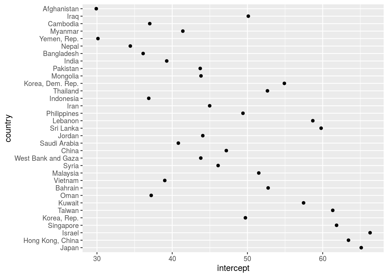
ggplot(gap_fitted, aes(x = slope, y = country)) +
  geom_point()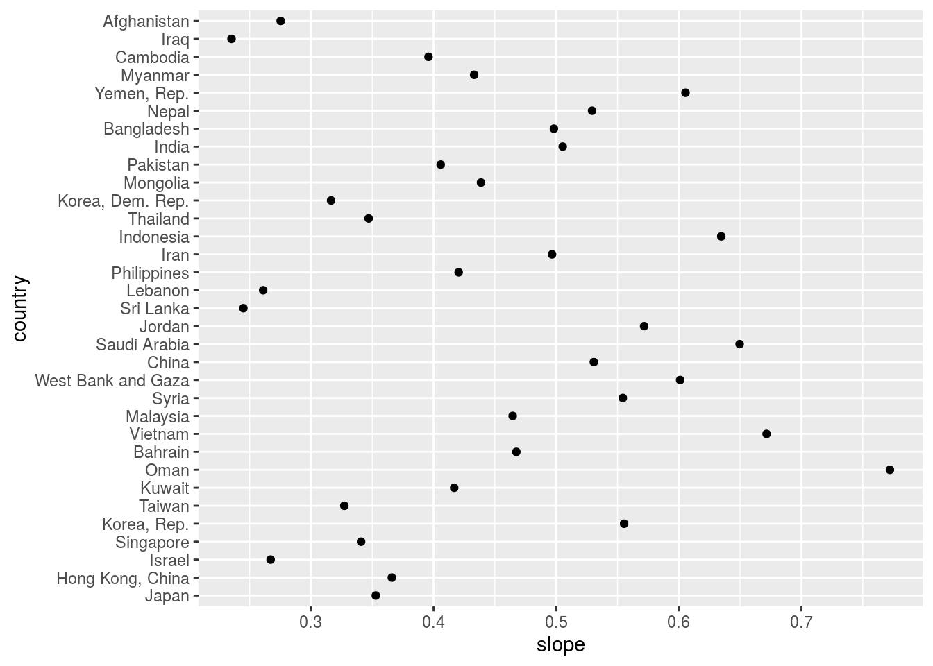
To get summary statistics implementing certain custom functions on list items. The case example below shows application of some high level functions available in tidyverse.
set.seed(1)

# construct a dataframe
d <- data_frame(n = c(5, 1, 3))
## Warning: `data_frame()` is deprecated as of tibble 1.1.0.
## Please use `tibble()` instead.
## This warning is displayed once every 8 hours.
## Call `lifecycle::last_warnings()` to see where this warning was generated.e <- d %>% group_by(n) %>%
do(data_frame(y = rnorm(.$n), dat = list(data.frame(a = 1))))
# this method is tranmutating type (drops original)
e %>% rowwise() %>% do(data_frame(sum = .$y + .$n))## Source: local data frame [9 x 1]
## Groups: <by row>
##
## # A tibble: 9 x 1
## sum
## * <dbl>
## 1 0.374
## 2 3.18
## 3 2.16
## 4 4.60
## 5 5.33
## 6 4.18
## 7 5.49
## 8 5.74
## 9 5.58# this only adds the mutated summary (keeps original)
mutate(e, sum = purrr::map2_dbl(y, n, `+`))## # A tibble: 9 x 4
## # Groups: n [3]
## n y dat sum
## <dbl> <dbl> <list> <dbl>
## 1 1 -0.626 <df[,1] [1 × 1]> 0.374
## 2 3 0.184 <df[,1] [1 × 1]> 3.18
## 3 3 -0.836 <df[,1] [1 × 1]> 2.16
## 4 3 1.60 <df[,1] [1 × 1]> 4.60
## 5 5 0.330 <df[,1] [1 × 1]> 5.33
## 6 5 -0.820 <df[,1] [1 × 1]> 4.18
## 7 5 0.487 <df[,1] [1 × 1]> 5.49
## 8 5 0.738 <df[,1] [1 × 1]> 5.74
## 9 5 0.576 <df[,1] [1 × 1]> 5.58# # .f should be able to work with a list or a data frame. As it
# happens, sum() handles data frame so the following works:
mtcars %>% purrrlyr::by_row(sum)## # A tibble: 32 x 12
## mpg cyl disp hp drat wt qsec vs am gear carb .out
## <dbl> <dbl> <dbl> <dbl> <dbl> <dbl> <dbl> <dbl> <dbl> <dbl> <dbl> <list>
## 1 21 6 160 110 3.9 2.62 16.5 0 1 4 4 <dbl [1]>
## 2 21 6 160 110 3.9 2.88 17.0 0 1 4 4 <dbl [1]>
## 3 22.8 4 108 93 3.85 2.32 18.6 1 1 4 1 <dbl [1]>
## 4 21.4 6 258 110 3.08 3.22 19.4 1 0 3 1 <dbl [1]>
## 5 18.7 8 360 175 3.15 3.44 17.0 0 0 3 2 <dbl [1]>
## 6 18.1 6 225 105 2.76 3.46 20.2 1 0 3 1 <dbl [1]>
## 7 14.3 8 360 245 3.21 3.57 15.8 0 0 3 4 <dbl [1]>
## 8 24.4 4 147. 62 3.69 3.19 20 1 0 4 2 <dbl [1]>
## 9 22.8 4 141. 95 3.92 3.15 22.9 1 0 4 2 <dbl [1]>
## 10 19.2 6 168. 123 3.92 3.44 18.3 1 0 4 4 <dbl [1]>
## # … with 22 more rows# # Other functions such as mean() may need to be adjusted with one
# # of the lift_xy() helpers:
mtcars %>% purrrlyr::by_row(purrr::lift_vl(mean))## # A tibble: 32 x 12
## mpg cyl disp hp drat wt qsec vs am gear carb .out
## <dbl> <dbl> <dbl> <dbl> <dbl> <dbl> <dbl> <dbl> <dbl> <dbl> <dbl> <list>
## 1 21 6 160 110 3.9 2.62 16.5 0 1 4 4 <dbl [1]>
## 2 21 6 160 110 3.9 2.88 17.0 0 1 4 4 <dbl [1]>
## 3 22.8 4 108 93 3.85 2.32 18.6 1 1 4 1 <dbl [1]>
## 4 21.4 6 258 110 3.08 3.22 19.4 1 0 3 1 <dbl [1]>
## 5 18.7 8 360 175 3.15 3.44 17.0 0 0 3 2 <dbl [1]>
## 6 18.1 6 225 105 2.76 3.46 20.2 1 0 3 1 <dbl [1]>
## 7 14.3 8 360 245 3.21 3.57 15.8 0 0 3 4 <dbl [1]>
## 8 24.4 4 147. 62 3.69 3.19 20 1 0 4 2 <dbl [1]>
## 9 22.8 4 141. 95 3.92 3.15 22.9 1 0 4 2 <dbl [1]>
## 10 19.2 6 168. 123 3.92 3.44 18.3 1 0 4 4 <dbl [1]>
## # … with 22 more rows# To run a function with invoke_rows(), make sure it is variadic (that
# it accepts dots) or that .f's signature is compatible with the
# column names
mtcars %>% purrrlyr::invoke_rows(.f = sum)## # A tibble: 32 x 12
## mpg cyl disp hp drat wt qsec vs am gear carb .out
## <dbl> <dbl> <dbl> <dbl> <dbl> <dbl> <dbl> <dbl> <dbl> <dbl> <dbl> <list>
## 1 21 6 160 110 3.9 2.62 16.5 0 1 4 4 <dbl [1]>
## 2 21 6 160 110 3.9 2.88 17.0 0 1 4 4 <dbl [1]>
## 3 22.8 4 108 93 3.85 2.32 18.6 1 1 4 1 <dbl [1]>
## 4 21.4 6 258 110 3.08 3.22 19.4 1 0 3 1 <dbl [1]>
## 5 18.7 8 360 175 3.15 3.44 17.0 0 0 3 2 <dbl [1]>
## 6 18.1 6 225 105 2.76 3.46 20.2 1 0 3 1 <dbl [1]>
## 7 14.3 8 360 245 3.21 3.57 15.8 0 0 3 4 <dbl [1]>
## 8 24.4 4 147. 62 3.69 3.19 20 1 0 4 2 <dbl [1]>
## 9 22.8 4 141. 95 3.92 3.15 22.9 1 0 4 2 <dbl [1]>
## 10 19.2 6 168. 123 3.92 3.44 18.3 1 0 4 4 <dbl [1]>
## # … with 22 more rowsmtcars %>% purrrlyr::invoke_rows(.f = purrr::lift_vd(mean))## # A tibble: 32 x 12
## mpg cyl disp hp drat wt qsec vs am gear carb .out
## <dbl> <dbl> <dbl> <dbl> <dbl> <dbl> <dbl> <dbl> <dbl> <dbl> <dbl> <list>
## 1 21 6 160 110 3.9 2.62 16.5 0 1 4 4 <dbl [1]>
## 2 21 6 160 110 3.9 2.88 17.0 0 1 4 4 <dbl [1]>
## 3 22.8 4 108 93 3.85 2.32 18.6 1 1 4 1 <dbl [1]>
## 4 21.4 6 258 110 3.08 3.22 19.4 1 0 3 1 <dbl [1]>
## 5 18.7 8 360 175 3.15 3.44 17.0 0 0 3 2 <dbl [1]>
## 6 18.1 6 225 105 2.76 3.46 20.2 1 0 3 1 <dbl [1]>
## 7 14.3 8 360 245 3.21 3.57 15.8 0 0 3 4 <dbl [1]>
## 8 24.4 4 147. 62 3.69 3.19 20 1 0 4 2 <dbl [1]>
## 9 22.8 4 141. 95 3.92 3.15 22.9 1 0 4 2 <dbl [1]>
## 10 19.2 6 168. 123 3.92 3.44 18.3 1 0 4 4 <dbl [1]>
## # … with 22 more rows# # invoke_rows() with cols collation is equivalent to plyr::mdply()
p <- expand.grid(mean = 1:5, sd = seq(0, 1, length = 10))
p %>% purrrlyr::invoke_rows(.f = rnorm, n = 5, .collate = "cols")## # A tibble: 50 x 7
## mean sd .out1 .out2 .out3 .out4 .out5
## <int> <dbl> <dbl> <dbl> <dbl> <dbl> <dbl>
## 1 1 0 1 1 1 1 1
## 2 2 0 2 2 2 2 2
## 3 3 0 3 3 3 3 3
## 4 4 0 4 4 4 4 4
## 5 5 0 5 5 5 5 5
## 6 1 0.111 0.966 1.17 1.04 0.931 0.754
## 7 2 0.111 2.12 2.00 2.00 2.10 2.09
## 8 3 0.111 3.07 3.10 3.09 3.01 2.78
## 9 4 0.111 4.07 3.99 3.98 3.84 3.95
## 10 5 0.111 5.05 5.15 4.99 5.04 4.99
## # … with 40 more rows# p %>% plyr::mdply(rnorm, n = 5) %>% dplyr::tbl_df()
# # To integrate the result as part of the data frame, use rows or
# # cols collation:
mtcars[1:2] %>% purrrlyr::by_row(function(x) 1:5)## # A tibble: 32 x 3
## mpg cyl .out
## <dbl> <dbl> <list>
## 1 21 6 <int [5]>
## 2 21 6 <int [5]>
## 3 22.8 4 <int [5]>
## 4 21.4 6 <int [5]>
## 5 18.7 8 <int [5]>
## 6 18.1 6 <int [5]>
## 7 14.3 8 <int [5]>
## 8 24.4 4 <int [5]>
## 9 22.8 4 <int [5]>
## 10 19.2 6 <int [5]>
## # … with 22 more rowsmtcars[1:2] %>% purrrlyr::by_row(function(x) 1:5, .collate = "rows")## # A tibble: 160 x 4
## mpg cyl .row .out
## <dbl> <dbl> <int> <int>
## 1 21 6 1 1
## 2 21 6 1 2
## 3 21 6 1 3
## 4 21 6 1 4
## 5 21 6 1 5
## 6 21 6 2 1
## 7 21 6 2 2
## 8 21 6 2 3
## 9 21 6 2 4
## 10 21 6 2 5
## # … with 150 more rowsmtcars[1:2] %>% purrrlyr::by_row(function(x) 1:5, .collate = "cols")## # A tibble: 32 x 7
## mpg cyl .out1 .out2 .out3 .out4 .out5
## <dbl> <dbl> <int> <int> <int> <int> <int>
## 1 21 6 1 2 3 4 5
## 2 21 6 1 2 3 4 5
## 3 22.8 4 1 2 3 4 5
## 4 21.4 6 1 2 3 4 5
## 5 18.7 8 1 2 3 4 5
## 6 18.1 6 1 2 3 4 5
## 7 14.3 8 1 2 3 4 5
## 8 24.4 4 1 2 3 4 5
## 9 22.8 4 1 2 3 4 5
## 10 19.2 6 1 2 3 4 5
## # … with 22 more rows# # getting custom summary functions with purrr and dplyr verbs
mtcars %>%
group_by(cyl) %>%
tidyr::nest() %>%
mutate(model = purrr::map(data, ~lm(qsec ~ hp, .)),
coef = purrr::map_dbl(model, ~coef(.)[2])) %>%
tidyr::unnest(data)## # A tibble: 32 x 13
## # Groups: cyl [3]
## cyl mpg disp hp drat wt qsec vs am gear carb model
## <dbl> <dbl> <dbl> <dbl> <dbl> <dbl> <dbl> <dbl> <dbl> <dbl> <dbl> <lis>
## 1 6 21 160 110 3.9 2.62 16.5 0 1 4 4 <lm>
## 2 6 21 160 110 3.9 2.88 17.0 0 1 4 4 <lm>
## 3 6 21.4 258 110 3.08 3.22 19.4 1 0 3 1 <lm>
## 4 6 18.1 225 105 2.76 3.46 20.2 1 0 3 1 <lm>
## 5 6 19.2 168. 123 3.92 3.44 18.3 1 0 4 4 <lm>
## 6 6 17.8 168. 123 3.92 3.44 18.9 1 0 4 4 <lm>
## 7 6 19.7 145 175 3.62 2.77 15.5 0 1 5 6 <lm>
## 8 4 22.8 108 93 3.85 2.32 18.6 1 1 4 1 <lm>
## 9 4 24.4 147. 62 3.69 3.19 20 1 0 4 2 <lm>
## 10 4 22.8 141. 95 3.92 3.15 22.9 1 0 4 2 <lm>
## # … with 22 more rows, and 1 more variable: coef <dbl># # run a regression after group_by operation
# # and save results to dataframe
group_by(mtcars, gear) %>% do(res = residuals(lm(mpg~carb, .)))## Source: local data frame [3 x 2]
## Groups: <by row>
##
## # A tibble: 3 x 2
## gear res
## * <dbl> <list>
## 1 3 <dbl [15]>
## 2 4 <dbl [12]>
## 3 5 <dbl [5]># # yet better way to capture the results -- residuals.
# # then it can be combined with original data.
mtcars %>%
group_by(cyl) %>%
do(model = lm(mpg ~ wt, data=.)) %>%
do((function(reg_mod) {
data.frame(reg_res = residuals(reg_mod$model))
})(.))## Source: local data frame [32 x 1]
## Groups: <by row>
##
## # A tibble: 32 x 1
## reg_res
## * <dbl>
## 1 -3.67
## 2 2.84
## 3 1.02
## 4 5.25
## 5 -0.0513
## 6 4.69
## 7 -4.15
## 8 -1.34
## 9 -1.49
## 10 -0.627
## # … with 22 more rows# # Custom data modeling
# # using dplyr do() calls
fertility <- read_csv("./data/fertility.csv")## Parsed with column specification:
## cols(
## AGE = col_double(),
## Year = col_double(),
## fertility = col_double()
## )# # binding predictions to original dataframe
fertility %>%
group_by(Year) %>%
do(data.frame(.,pred = predict(mgcv::gam(fertility ~ s(AGE), data=.))))## # A tibble: 60 x 4
## # Groups: Year [2]
## AGE Year fertility pred
## <dbl> <dbl> <dbl> <dbl>
## 1 15 1930 5.17 -0.828
## 2 16 1930 14.2 16.2
## 3 17 1930 27.7 33.4
## 4 18 1930 44.6 51.1
## 5 19 1930 59.1 69.2
## 6 20 1930 89.7 87.3
## 7 21 1930 105. 104.
## 8 22 1930 120. 120.
## 9 23 1930 137. 132.
## 10 24 1930 149. 141.
## # … with 50 more rows# # same but different approach
do.call(rbind,
lapply(split(fertility, fertility$Year), function(df) {
df$pred <- predict(mgcv::gam(fertility ~ s(AGE), data=df))
df
}))## # A tibble: 60 x 4
## AGE Year fertility pred
## * <dbl> <dbl> <dbl> <dbl>
## 1 15 1930 5.17 -0.828
## 2 16 1930 14.2 16.2
## 3 17 1930 27.7 33.4
## 4 18 1930 44.6 51.1
## 5 19 1930 59.1 69.2
## 6 20 1930 89.7 87.3
## 7 21 1930 105. 104.
## 8 22 1930 120. 120.
## 9 23 1930 137. 132.
## 10 24 1930 149. 141.
## # … with 50 more rows# # same using data.table library
fertility %>%
data.table::data.table() %>%
group_by(Year) %>%
mutate(pred = predict(mgcv::gam(fertility ~ s(AGE))))## # A tibble: 60 x 4
## # Groups: Year [2]
## AGE Year fertility pred
## <dbl> <dbl> <dbl> <dbl>
## 1 15 1930 5.17 -0.828
## 2 16 1930 14.2 16.2
## 3 17 1930 27.7 33.4
## 4 18 1930 44.6 51.1
## 5 19 1930 59.1 69.2
## 6 20 1930 89.7 87.3
## 7 21 1930 105. 104.
## 8 22 1930 120. 120.
## 9 23 1930 137. 132.
## 10 24 1930 149. 141.
## # … with 50 more rows# # this fails at last line
# fertility %>%
# group_by(Year) %>%
# dplyr::do(model = mgcv::gam(fertility ~ s(AGE), data = .)) %>%
# left_join(fertility, .) %>%
# mutate(smoothed = predict(model, newdata = AGE))
# # multiple model fitting and parameter extraction
fitmodel <- function(d) lm(mpg ~ disp, data = mtcars)
by_cyl <- mtcars %>%
group_by(cyl) %>%
tidyr::nest() %>%
mutate(mod = purrr::map(data, fitmodel),
pars = purrr::map(mod, broom::tidy),
pred = purrr::map(mod, broom::augment))
pars <- by_cyl %>% tidyr::unnest(pars)
pars## # A tibble: 6 x 9
## # Groups: cyl [3]
## cyl data mod term estimate std.error statistic p.value pred
## <dbl> <list> <lis> <chr> <dbl> <dbl> <dbl> <dbl> <list>
## 1 6 <tibble [… <lm> (Inter… 29.6 1.23 24.1 3.58e-21 <tibble …
## 2 6 <tibble [… <lm> disp -0.0412 0.00471 -8.75 9.38e-10 <tibble …
## 3 4 <tibble [… <lm> (Inter… 29.6 1.23 24.1 3.58e-21 <tibble …
## 4 4 <tibble [… <lm> disp -0.0412 0.00471 -8.75 9.38e-10 <tibble …
## 5 8 <tibble [… <lm> (Inter… 29.6 1.23 24.1 3.58e-21 <tibble …
## 6 8 <tibble [… <lm> disp -0.0412 0.00471 -8.75 9.38e-10 <tibble …prediction <- by_cyl %>% tidyr::unnest(pred)
prediction## # A tibble: 96 x 14
## # Groups: cyl [3]
## cyl data mod pars .rownames mpg disp .fitted .se.fit .resid .hat
## <dbl> <lis> <lis> <lis> <chr> <dbl> <dbl> <dbl> <dbl> <dbl> <dbl>
## 1 6 <tib… <lm> <tib… Mazda RX4 21 160 23.0 0.664 -2.01 0.0418
## 2 6 <tib… <lm> <tib… Mazda RX… 21 160 23.0 0.664 -2.01 0.0418
## 3 6 <tib… <lm> <tib… Datsun 7… 22.8 108 25.1 0.815 -2.35 0.0629
## 4 6 <tib… <lm> <tib… Hornet 4… 21.4 258 19.0 0.589 2.43 0.0328
## 5 6 <tib… <lm> <tib… Hornet S… 18.7 360 14.8 0.838 3.94 0.0663
## 6 6 <tib… <lm> <tib… Valiant 18.1 225 20.3 0.575 -2.23 0.0313
## 7 6 <tib… <lm> <tib… Duster 3… 14.3 360 14.8 0.838 -0.462 0.0663
## 8 6 <tib… <lm> <tib… Merc 240D 24.4 147. 23.6 0.698 0.846 0.0461
## 9 6 <tib… <lm> <tib… Merc 230 22.8 141. 23.8 0.714 -0.997 0.0482
## 10 6 <tib… <lm> <tib… Merc 280 19.2 168. 22.7 0.647 -3.49 0.0396
## # … with 86 more rows, and 3 more variables: .sigma <dbl>, .cooksd <dbl>,
## # .std.resid <dbl>Workarounds on unequal length lists
hareramshyam <- list(harry = c(1, 2, 3, 4, 5), ram = c(2, 3, 4, 6, 8), shyam = c(3, 4, 5, 3, 2, 4, 5, 6, 3))

## binding rows for two list items of equal lengths is possible
bind_rows(hareramshyam[1:2])
## # A tibble: 5 x 2
## harry ram
## <dbl> <dbl>
## 1 1 2
## 2 2 3
## 3 3 4
## 4 4 6
## 5 5 8# bind_rows(hareramshyam) ## this fails
## so to complete the list by filling with nas to match the
## length of each element in list, use
mymax <- hareramshyam %>%
lapply(length) %>%
unlist %>%
max
hareramshyam %>%
lapply(function(x) c(x, rep(NA_integer_, mymax-length(x)))) %>%
bind_rows()## # A tibble: 9 x 3
## harry ram shyam
## <dbl> <dbl> <dbl>
## 1 1 2 3
## 2 2 3 4
## 3 3 4 5
## 4 4 6 3
## 5 5 8 2
## 6 NA NA 4
## 7 NA NA 5
## 8 NA NA 6
## 9 NA NA 3## here is a two liner that could be cause the same
lapply(hareramshyam, `length<-`,
max(lengths(hareramshyam))) %>%
bind_rows()## # A tibble: 9 x 3
## harry ram shyam
## <dbl> <dbl> <dbl>
## 1 1 2 3
## 2 2 3 4
## 3 3 4 5
## 4 4 6 3
## 5 5 8 2
## 6 NA NA 4
## 7 NA NA 5
## 8 NA NA 6
## 9 NA NA 3# or use plyr's binder to avoid recycling
plyr::rbind.fill(map(hareramshyam, ~ as.data.frame(t(.x),stringsAsFactors=FALSE)))## V1 V2 V3 V4 V5 V6 V7 V8 V9
## 1 1 2 3 4 5 NA NA NA NA
## 2 2 3 4 6 8 NA NA NA NA
## 3 3 4 5 3 2 4 5 6 3## to fill, for example above, dataframe of NAs with other
## elements of the dataframe
lapply(hareramshyam, `length<-`,
max(lengths(hareramshyam))) %>%
bind_rows() %>%
mutate(harry = dplyr::coalesce(harry, shyam),
ram = dplyr::coalesce(ram, shyam))## # A tibble: 9 x 3
## harry ram shyam
## <dbl> <dbl> <dbl>
## 1 1 2 3
## 2 2 3 4
## 3 3 4 5
## 4 4 6 3
## 5 5 8 2
## 6 4 4 4
## 7 5 5 5
## 8 6 6 6
## 9 3 3 3Quick saving dataframe as image/vector
df <- augd[augd %>% str_detect("age$") %>% # augd is a character vector
             which()] %>%
  tibble() %>%
  split(f = as.factor(rep(1:4))) %>%
  bind_cols() %>%
  magrittr::set_colnames(paste0("shitlist", 1:4))

# png("./shitlist.png", height = 22*nrow(df), width = 100*ncol(df))
# grid.table(df)
# dev.off()
The dataframe can be quickly saved as image by:
png("./shitlist.png", height = 22*nrow(df), width = 100*ncol(df))
grid.table(df)
dev.off()