The birthday problem: Non analytical solution

# Birthday problem

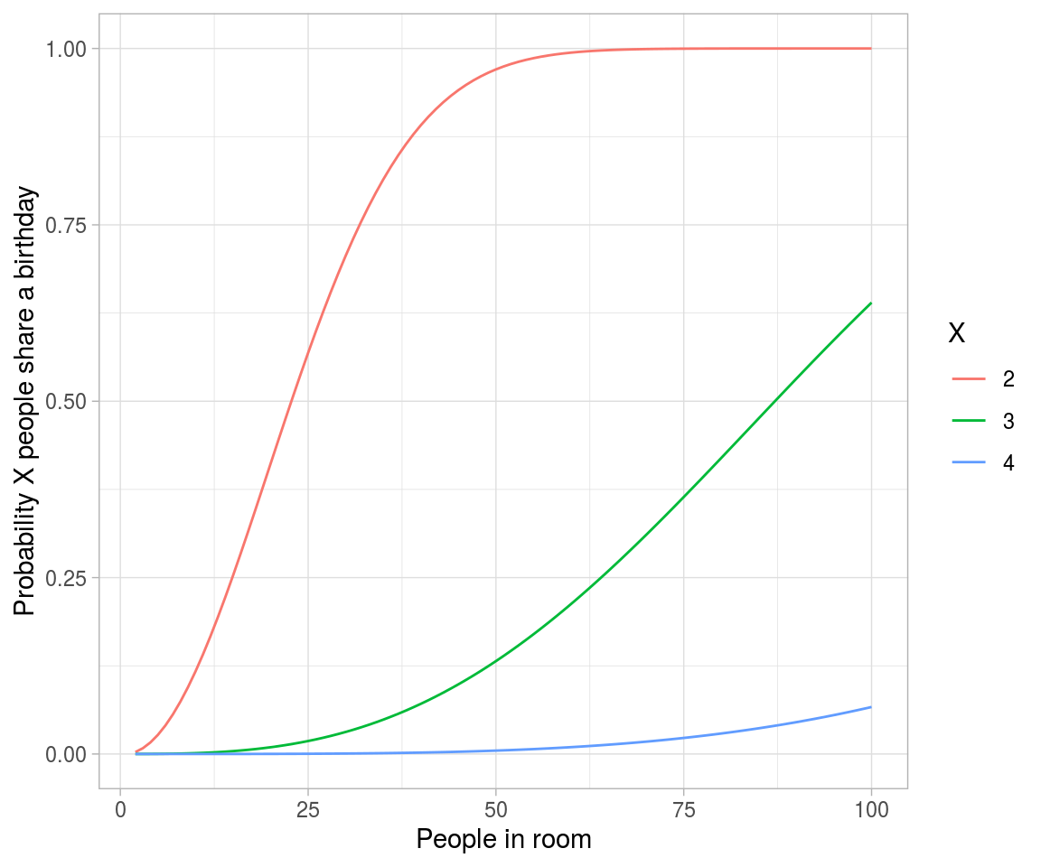
crossing(n = 2:100, 
         x = 2:4) %>% 
  mutate(probability = map2_dbl(n, x, ~pbirthday(.x, coincident = .y))) %>% 
  ggplot(aes(n, probability, color = factor(x))) +
  geom_line() +
  labs(x = "People in room", 
       y = "Probability X people share a birthday", 
       color = "X")

# Approximating birthday paradox with Poisson distribution

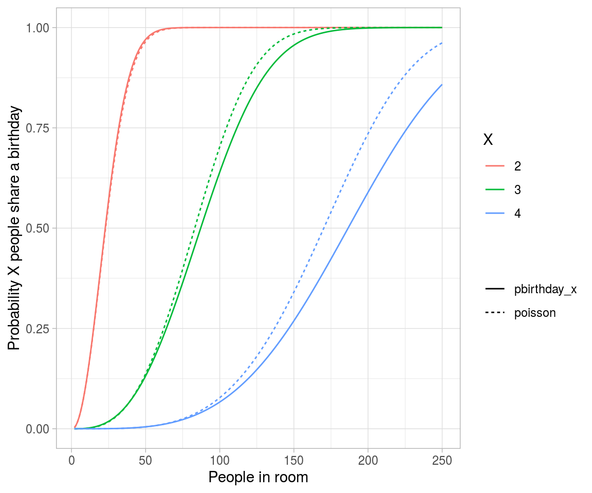
crossing(n = 2:250, 
         x = 2:4) %>% 
  mutate(combinations = choose(n, x), 
         probability_each = (1/365)^(x-1), 
         poisson = 1-dpois(0, combinations * probability_each), 
         pbirthday_x = map2_dbl(n, x, ~pbirthday(.x, coincident = .y))) %>% 
  gather(type, probability, pbirthday_x, poisson) %>% 
  ggplot(aes(n, probability, color = factor(x), lty = type)) +
  geom_line() +
  labs(x = "People in room", 
       y = "Probability X people share a birthday", 
       color = "X", 
       lty = "")

# the reason is because events are no longer weakly dependent-every pair makes triplets
# more likely.

# Analytical solution to birthday problem (Mikhail Papov; bearlogic.github.io)

# Suppose, we are interested in the probability that, in a set of n randomly chosen people, some pair of them will have the same
# birthday (which we refer to as event A).

# Using Kolmogorov axionms and conditional probability, we can derive an analytical solution for P(A):

# P(A) = 1-\frac{n!.\binom{365}{n}}{365^n}

# This can be solved in `R` as:

pa <- function(n){
  1 - (factorial(n) * choose(365, n))/(365^n)
}

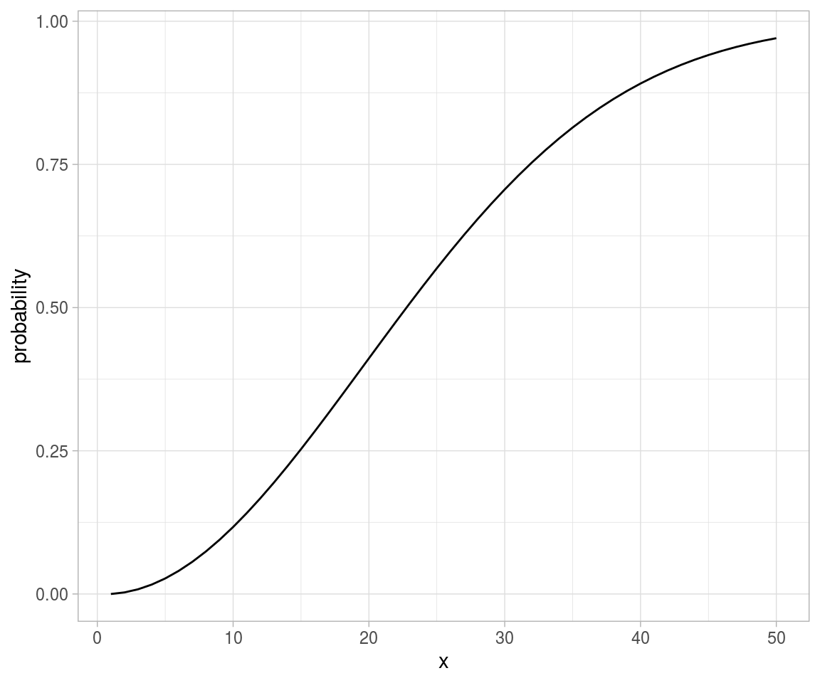
map_dfr(.x = list(probability = 1:50), .f = pa) %>% 
  mutate(x = seq_along(probability)) %>% 
  ggplot(aes(x = x, y = probability)) +
  geom_line()