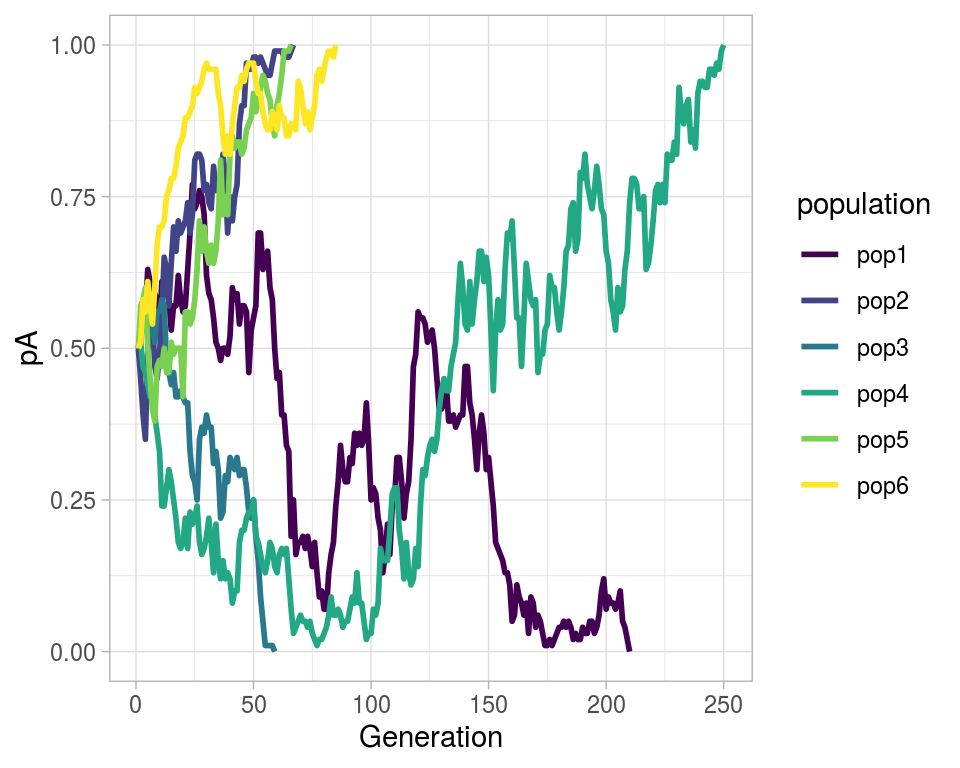
Simulating genetic drift

Genetic drift is the result of bernouli process on survival of individuals (given some probability for each of them) of a population over a number of independent trials (Generation).

Apparently there are two techniques of seeing such process – one individual level, other the population level. Both solutions are illustrated below. Let us suppose population of N individuals remains fixed from generation to generation, likewise, Fitness probability of “A” allele (\(p(A)\)) and “a” allele (\(p(a)\)) both starts off equal. Now we can generate incremental population survival probability for each individual for given population size:

N <- 100
pA <- vector()
pA[1] <- 0.5
i <- 1

while ((pA[i] < 1) & (pA[i] > 0)) {
  nA <- 0

  for (j in 1:N){
    random <- runif(1)
    if(random < pA[i]){nA <- nA + 1}
  }
  pA[i + 1] <- nA/N
  i <- i + 1
}

Alternatively rbinom function generates the same but with probabilistic draw from entire population.

drift_generate <- function(N = 100){
  N <- N
  pA <- vector()
  pA[1] <- 0.5
  i <- 1
  
  while ((pA[i] < 1) & (pA[i] > 0)) {
    nA <- rbinom(n = 1, size = N, prob = pA[i])
    pA[i + 1] <- nA/N
    i <- i + 1
  }
  return(tidyr::tibble(i = 1:i, pA = pA))
}

drift_tibble <- purrr::map_dfr(c(pop1 = 1, pop2 = 2, 
                                 pop3 = 3, pop4 = 4, 
                                 pop5 = 5, pop6 = 6), 
                               ~drift_generate(N = 100), .id = "population")

drift_gg <- ggplot(aes(x = i, y = pA), data = drift_tibble) +
  # geom_point(aes(color = population)) +
  geom_path(aes(color = population), size = 1.0) +
  theme_light() +
  scale_color_viridis_d() +
  labs(x = "Generation")

drift_gg