A normal function isn’t so normal

The normal density function is:

\[ \large f(x) = \frac{1}{\sqrt{2 \pi} \sigma} \exp^{-\frac{(x - \mu)^2}{(2 \sigma^2)}} \]

It doesn’t make sense to calculate the probability for a single value in a continuous probability function, it is by definition zero, but you can calculate relative likelihoods (heights). dnorm simply gives the value of the function for a given x, not the area under the curve for that x (which is basically nothing for a single value). To find the density (height) for a single x value on the normal distribution, use dnorm() in the following way (here each x value is treated as separate and vectorized over),

https://stackoverflow.com/questions/57345406/estimating-probability-density-in-a-range-between-two-x-values-on-simulated-data

example_data <- c(0.2, 1.2, 1.2, 1.4, 1.5, 1.3, 1.2, 1.3, 1.6, 1.9, 2.3)

dnorm(example_data, mean = 0, sd = 1)

##  [1] 0.39104269 0.19418605 0.19418605 0.14972747 0.12951760 0.17136859
##  [7] 0.19418605 0.17136859 0.11092083 0.06561581 0.02832704

normal_density <- function(x, mu=0, sd=1){1/(sqrt(2 * pi)*sd) * exp(-((x - mu)^2/(2 * sd^2)))}
normal_density(example_data, mu = 0, sd = 1)

##  [1] 0.39104269 0.19418605 0.19418605 0.14972747 0.12951760 0.17136859
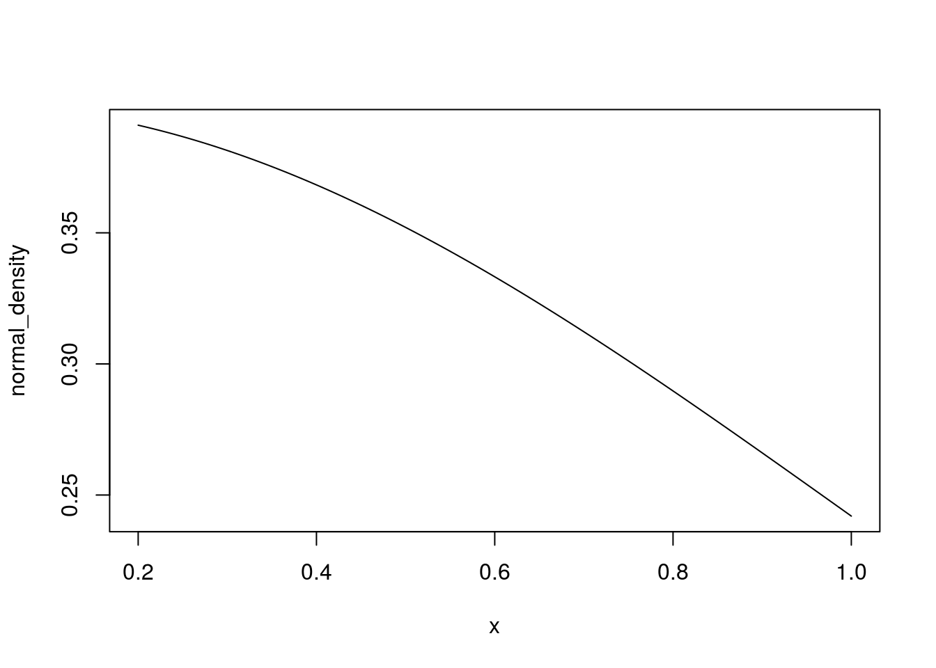
##  [7] 0.19418605 0.17136859 0.11092083 0.06561581 0.02832704

plot.function(normal_density, from = example_data)

It is also possible to obtain approximate probability density function using density and approxfun

estimated_dfun <- approxfun(density(example_data), rule=2)

From the estimated density function point probability density estimates could be made as:

estimated_dfun(1.45) # use any number to find the height ?

## [1] 1.083488

# the area under the curve:
area_under <- function(lower, upper) {
    integrate(estimated_dfun, lower=lower, upper=upper) }

ecdf() is the way to go for a non-parametric estimate, but if you expect a normal distribution you can also do a parametric estimate.

dist_mean <- 10
dist_sd <- 0.2
a <- 9.7
b <- 10.2

set.seed(123)
r <- rnorm(1e4, dist_mean, dist_sd)

# population
pnorm(b, dist_mean, dist_sd) - pnorm(a, dist_mean, dist_sd)

## [1] 0.7745375

# [1] 0.7745375

# parametric estimate
pnorm(b, mean(r), sd(r)) - pnorm(a, mean(r), sd(r))

## [1] 0.7753985

# [1] 0.7753985

# nonparametric estimate
ecdfun <- ecdf(r)
ecdfun(b) - ecdfun(a)

## [1] 0.7754

# [1] 0.7754