Logistic Regression: Part II - Varietal adoption dataset
Binary classifier using categorical predictor
Let’s say we have two variable – survey response of farmer to willingness to adopt improved rice variety (in YES/NO) and them having been trained earlier about agricultural input management (in trained/untrained).
Read in the data and notice the summary.
rice_data <- readxl::read_xlsx(here::here("content", "post", "data", "rice_variety_adoption.xlsx")) %>%
  mutate_if(.predicate = is.character, as.factor)

rice_variety_adoption <- readxl::read_xlsx(here::here("content", "post", "data", "rice_variety_adoption.xlsx")) %>%
  select(improved_variety_adoption, training) %>%
  # convert data to suitable factor type for analysis.
  mutate_if(is.character, as.factor)

head(rice_variety_adoption) # now we have data
## # A tibble: 6 x 2
## improved_variety_adoption training
## <fct> <fct>
## 1 No No
## 2 Yes No
## 3 No No
## 4 Yes No
## 5 Yes No
## 6 No NoAs a basic descriptive, contruct one way and two way cross tabulation summary, showing count of each categories. This is because logistic regression uses count data, much like in a non-parametric model.
# count the data in a one way and two way tabulation
rice_variety_adoption %>% # fortunately there are no rare class (i.e. some class have exceptionally low frequencies)
  count(improved_variety_adoption)
## # A tibble: 2 x 2
## improved_variety_adoption n
## <fct> <int>
## 1 No 18
## 2 Yes 42rice_variety_adoption %>% # fortunately there are no rare class (i.e. some class have exceptionally low frequencies)
count(training)## # A tibble: 2 x 2
## training n
## <fct> <int>
## 1 No 43
## 2 Yes 17# # two way cross tabs
# rice_variety_adoption %>%
# count(improved_variety_adoption, training) %>%
# tidyr::pivot_wider(id_cols = improved_variety_adoption:training,
# names_from = training, values_from = n)
# two way cross tabs (confusion matrix) using yardstick
yardstick::conf_mat(table(rice_variety_adoption)) # class: conf_mat## training
## improved_variety_adoption No Yes
## No 17 1
## Yes 26 16The data representation quickly shows that most of the non adopters have not received training 17, compared to non-adopters that have received training 1. Similarly, the odds that a farmer will be a non adopter if he is trained versus untrained is: 1/17(too low); while the odds that a farmer will be an adopter if he is trained versus untrained is: 16/26 (relatively high).
To statistically verify, we formuate a generalized linear model that uses training to predict adoption of improved variety.
rice_glm <- glm(improved_variety_adoption ~ training, data = rice_variety_adoption, family = "binomial")
rice_glm %>% summary()
##
## Call:
## glm(formula = improved_variety_adoption ~ training, family = "binomial",
## data = rice_variety_adoption)
##
## Deviance Residuals:
## Min 1Q Median 3Q Max
## -2.3804 -1.3623 0.3482 1.0031 1.0031
##
## Coefficients:
## Estimate Std. Error z value Pr(>|z|)
## (Intercept) 0.4249 0.3119 1.362 0.1731
## trainingYes 2.3477 1.0769 2.180 0.0293 *
## ---
## Signif. codes: 0 '***' 0.001 '**' 0.01 '*' 0.05 '.' 0.1 ' ' 1
##
## (Dispersion parameter for binomial family taken to be 1)
##
## Null deviance: 73.304 on 59 degrees of freedom
## Residual deviance: 65.319 on 58 degrees of freedom
## AIC: 69.319
##
## Number of Fisher Scoring iterations: 5The intercept is the log(odds) an untrained farmer will adopt the technolgy. This is because the “No” is the first factor in training variable. The odds is not significant; meaning that odds that an untrained farmer will adopt technology is not different from zero. This can be directly derived as: 26/17 = 1.5294118
The coefficient on training variable is significant and positive. This means that receiving training increases the odds of a farmer being an adopter significantly. Numerically, odds of being an adopter farmer are, on a log scale, 1.619 greater if the famerhas received a training. This can be directly derived as: log((17/1) / (26/16)) = 10.4615385
Now, we can calculate the overall “Pseudo R-squared” and its p-value. For logistic regression,
## NOTE: Since we are doing logistic regression...
## Null devaince = 2*(0 - LogLikelihood(null model))
##               = -2*LogLikihood(null model)
## Residual deviacne = 2*(0 - LogLikelihood(proposed model))
##                   = -2*LogLikelihood(proposed model)
ll.null <- rice_glm$null.deviance/-2
ll.proposed <- rice_glm$deviance/-2

## McFadden's Pseudo R^2 = [ LL(Null) - LL(Proposed) ] / LL(Null)
(ll.null - ll.proposed) / ll.null
## [1] 0.1089217Likewise based on \(\chi^2\) values, we can arrive at p-values.
## chi-square value = 2*(LL(Proposed) - LL(Null))
## p-value = 1 - pchisq(chi-square value, df = 2-1)
1 - pchisq(2*(ll.proposed - ll.null), df=1)
## [1] 0.0047183031 - pchisq((rice_glm$null.deviance - rice_glm$deviance), df=1)## [1] 0.004718303I is also informative to see in terms of what this logistic regression predicts, given that a farmer is either trained or untrained (and no other data about them).
rice_predicted <- tibble(
  probability_of_adoption=rice_glm$fitted.values,
  training=rice_variety_adoption$training)

## We can plot the data...
ggplot(data=rice_predicted, aes(x=training, y=probability_of_adoption)) +
  geom_point(aes(color=training), size=5) +
  xlab("Training") +
  ylab("Predicted probability of a farmer being an adopter") +
  theme_bw()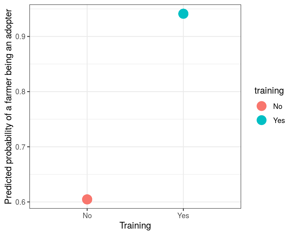
Since there are only two probabilities of adopting/non-adopting (one for trained and one for untrained), we can use a table to summarize the predicted probabilities.
xtabs(~ probability_of_adoption + training, data=rice_predicted)## training
## probability_of_adoption No Yes
## 0.604651162790698 43 0
## 0.941176470569947 0 17In a similar way multiple variables can be used as regressors to predict probability of farmer being an adopter of improved variety
Continuous predictor
rice_variety_adoption <- glm(improved_variety_adoption ~ farm_size, data = rice_data, family = binomial())

# also note that continuous response variables may infact be resulting form composite distributions

rice_data %>%
  ggplot() +
  geom_boxplot(aes(improved_variety_adoption, farm_size, fill = improved_variety_adoption), alpha = 0.6) +
  geom_violin(aes(improved_variety_adoption, farm_size, fill = improved_variety_adoption), alpha = 0.6) +
  scale_fill_discrete(guide = FALSE)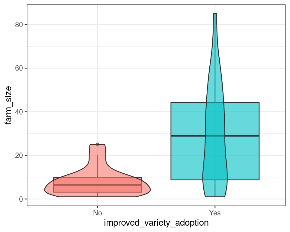
# break down globulin data into based on arbitrary value of 32
# check if the distribution is normal ?
rice_data %>%
  ggplot() +
  geom_density_ridges(aes(x = farm_size, y = training, fill = improved_variety_adoption),
              position = "identity",
              alpha = 0.6, scale = 1.1, rel_min_height = 0.05) + # `rel_min_height` is minimum height of density below which is ignored in display
  scale_fill_discrete(guide = FALSE)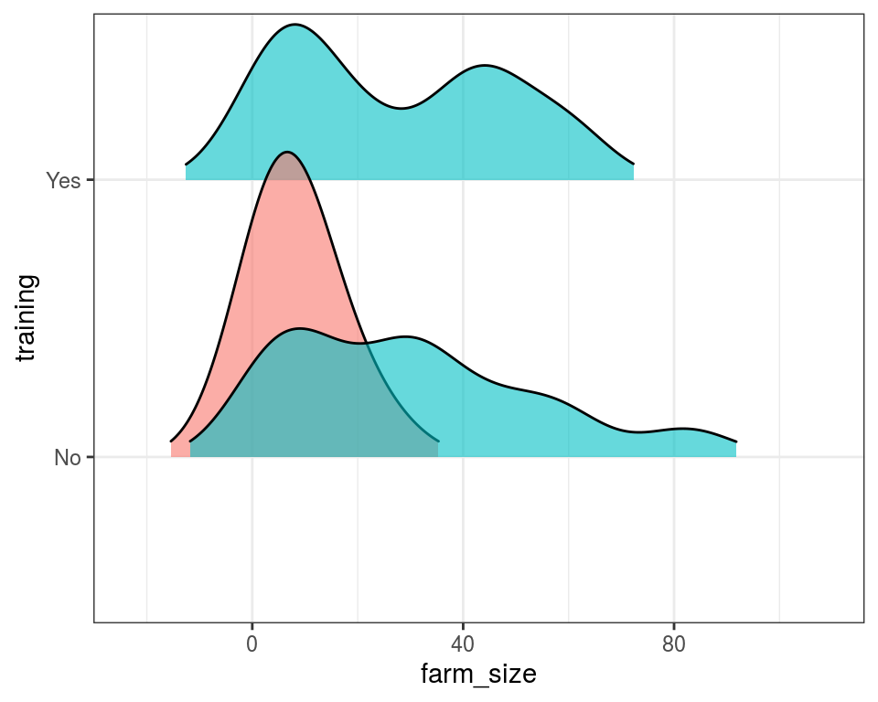
There is likely a presence of two peaks in the category receiving training.
rice_freq_tab_char <- rice_data %>%
  select_if(.predicate = function(x)is.character(x)|is.factor(x))

rice_freq_tab_char <- rice_freq_tab_char %>%
  pivot_longer(household_head_gender:last_col(), names_to = 'categorical_vars', values_to = "var_value") %>%
  group_by(categorical_vars, var_value) %>%
  count(sort = F) %>%
  ungroup()
Pie charts of all categorical variables.
rice_freq_tab_split <- rice_freq_tab_char %>%
  group_split(categorical_vars) %>%
  set_names(map(., ~unique(.x$categorical_vars)))

fpie <- map2(.x = rice_freq_tab_split,
             .y = names(rice_freq_tab_split),
             .f = ~ ggplot(.x,
                           aes(x="", y=n, fill=var_value)) +
               geom_bar(stat="identity", width=1) +
               # Convert to pie (polar coordinates) and add labels
               coord_polar("y", start=0) +
               ggrepel::geom_text_repel(aes(label = scales::percent(round(n/sum(n), 2))),
                         position = position_stack(vjust = 0.5), size = 4) +
               # Add color scale (hex colors)
               # scale_fill_manual(values=c("#55DDE0", "#33658A", "#2F4858",
               #                            "#F6AE2D", "#F26419")) +
               # use fill_viridis_d() for discrete values
               scale_fill_viridis_d(na.value = "grey50") +
               # faceting will add label to individual plot at least
               # facet_wrap(~`Socio-economic variables`) +
               # Remove labels and add title
               labs(x = NULL, y = NULL,
                    fill = NULL,
                    title = str_to_sentence(str_replace_all(.y, "_", " "))) +
               # Tidy up the theme
               theme_classic() +
               theme(axis.line = element_blank(),
                     axis.text = element_blank(),
                     axis.ticks = element_blank(),
                     plot.title = element_text(hjust = 0.5, color = "#666666"))
)

fpie
## $age_group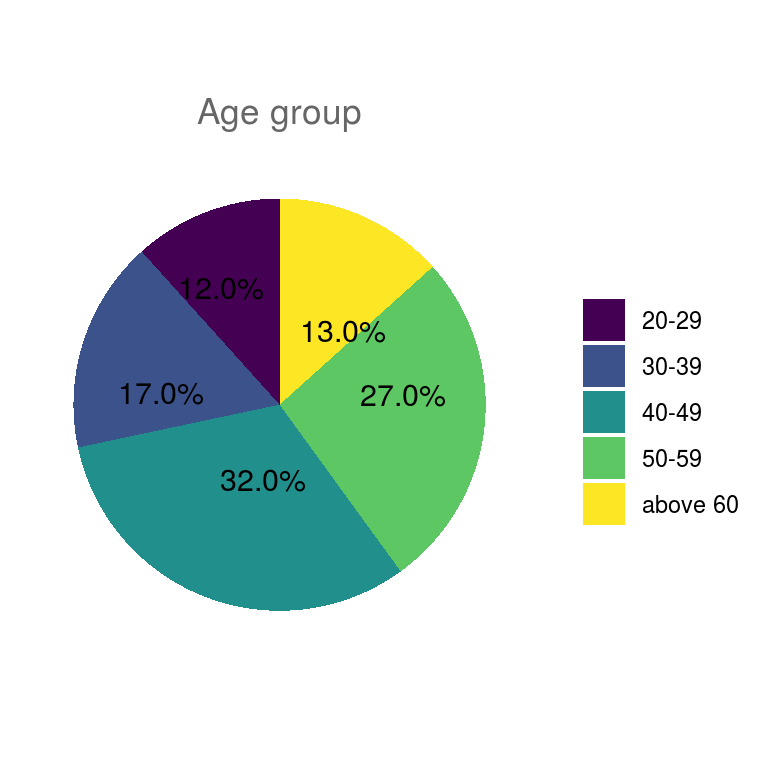
##
## $education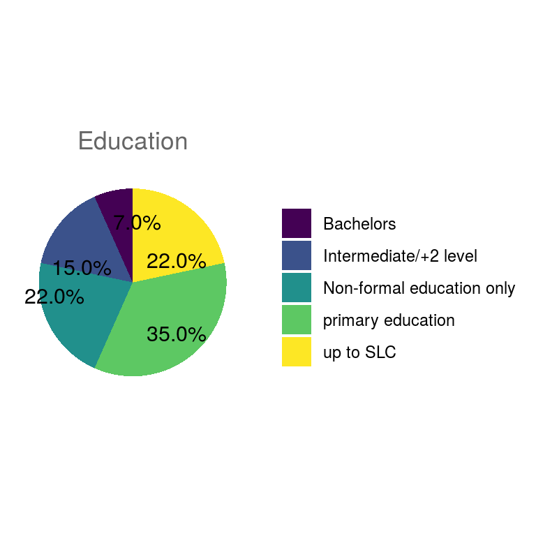
##
## $household_head_gender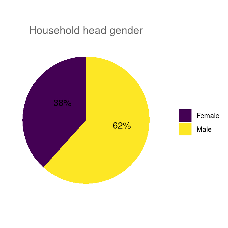
##
## $improved_variety_adoption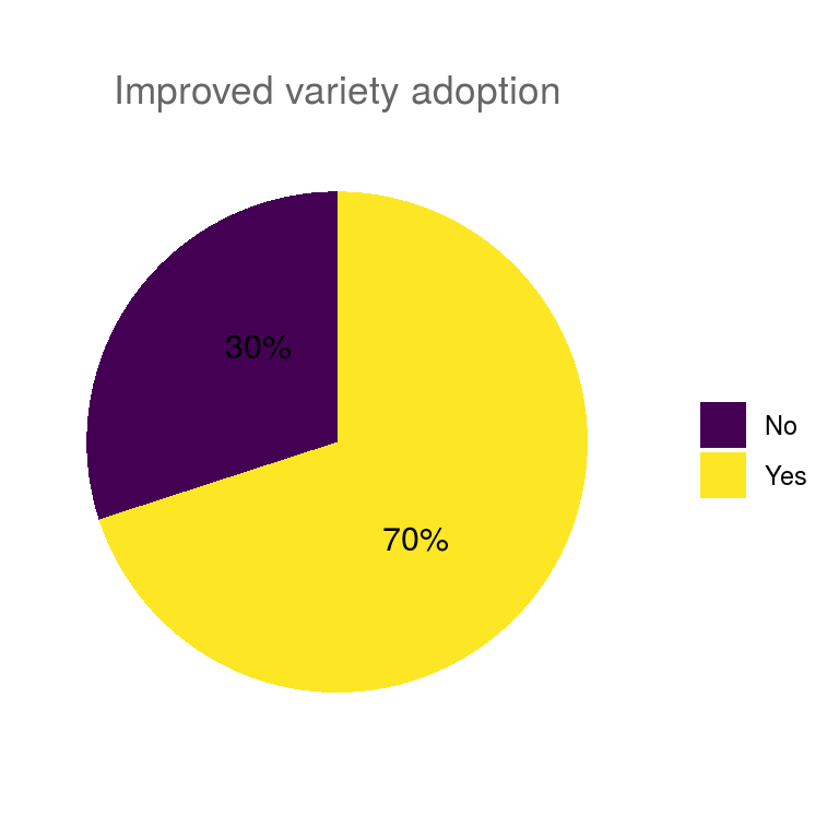
##
## $land_size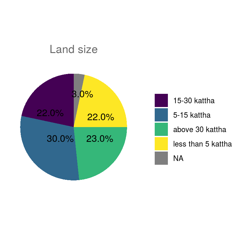
##
## $other_income_source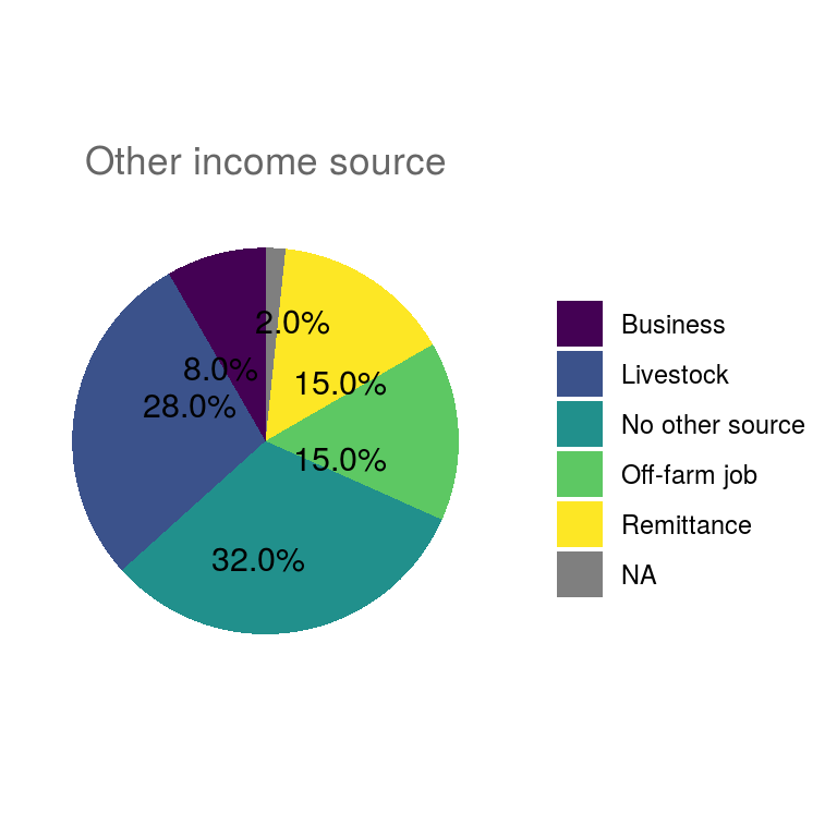
##
## $training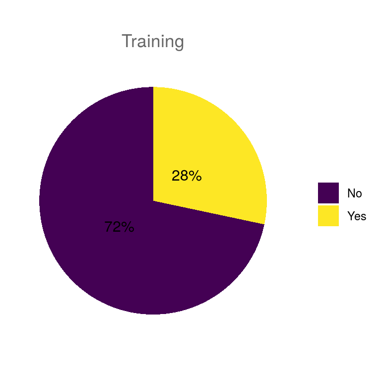
# # arrange pie plots in grid
# # grid.arrange(grobs = fpie, ncol = 3,
# #              top = "Percentage of response category for socio-economic variables in household samples") ## display plot
# ggsave(filename = "./socio_economic_pie.png",
#        arrangeGrob(grobs = fpie, ncol = 3,
#                    top = "Percentage of response category for categorical variables from surveyed households"),
#        width = 18, height = 18, device = "png", dpi = 300) ## save plot
Aggregating grouped variables for regression modeling.
# rice_data %>% skimr::skim()

rice_data_na_deselected <- rice_data %>%
  select(-shared_landsize, -irrigated_land_size) %>% # shared_landsize and irrigated_land_size both are continuous and have only 0.37, 0.67 complete
  mutate_if(is.character, as.factor)

# collapse factors
rice_data_na_deselected <- rice_data_na_deselected %>%
  mutate(other_income_source = fct_collapse(fct_explicit_na(other_income_source, na_level = "No"),
                                            Yes = c("Business", "Livestock", "Off-farm job", "Remittance"),
                                            No = c("No other source"))) %>%
  mutate(age_group = fct_collapse(age_group, "20-39" = c("20-29", "30-39"), ">=40" = c("40-49", "50-59", "above 60"))) %>%
  mutate(land_size = fct_collapse(land_size, "5-15 kattha" = c("5-15 kattha", "5-15 Kattha"))) %>%
  mutate(education = fct_collapse(education,
                                  "Primary or informal" = c("primary education", "Non-formal education only"),
                                  "Upto 10th" = c("up to SLC"),
                                  "Intermediate or higher" = c("Intermediate/+2 level", "Bachelors")))

rice_data_na_deselected %>% skimr::skim()| Name | Piped data |
| Number of rows | 60 |
| Number of columns | 10 |
| _______________________ | |
| Column type frequency: | |
| factor | 7 |
| numeric | 3 |
| ________________________ | |
| Group variables |
Variable type: factor
| skim_variable | n_missing | complete_rate | ordered | n_unique | top_counts |
|---|---|---|---|---|---|
| household_head_gender | 0 | 1.00 | FALSE | 2 | Mal: 37, Fem: 23 |
| age_group | 0 | 1.00 | FALSE | 2 | >=4: 43, 20-: 17 |
| education | 0 | 1.00 | FALSE | 3 | Pri: 34, Int: 13, Upt: 13 |
| land_size | 2 | 0.97 | FALSE | 4 | 5-1: 18, abo: 14, 15-: 13, les: 13 |
| other_income_source | 0 | 1.00 | FALSE | 2 | Yes: 40, No: 20 |
| improved_variety_adoption | 0 | 1.00 | FALSE | 2 | Yes: 42, No: 18 |
| training | 0 | 1.00 | FALSE | 2 | No: 43, Yes: 17 |
Variable type: numeric
| skim_variable | n_missing | complete_rate | mean | sd | p0 | p25 | p50 | p75 | p100 | hist |
|---|---|---|---|---|---|---|---|---|---|---|
| id | 0 | 1 | 30.50 | 17.46 | 1 | 15.75 | 30.5 | 45.25 | 60 | ▇▇▇▇▇ |
| family_size | 0 | 1 | 6.07 | 2.11 | 3 | 4.00 | 6.0 | 7.00 | 12 | ▇▇▇▂▁ |
| farm_size | 0 | 1 | 22.72 | 21.46 | 1 | 6.00 | 13.5 | 38.88 | 85 | ▇▂▂▁▁ |
GLM fit
rice_glm_fit <- glm(formula = improved_variety_adoption ~
                      household_head_gender +
                      age_group +
                      education +
                      land_size +
                      other_income_source +
                      improved_variety_adoption +
                      training +
                      family_size +
                      farm_size,
                    data = rice_data_na_deselected, family = "binomial")
rice_glm_fit %>%
  summary()
##
## Call:
## glm(formula = improved_variety_adoption ~ household_head_gender +
## age_group + education + land_size + other_income_source +
## improved_variety_adoption + training + family_size + farm_size,
## family = "binomial", data = rice_data_na_deselected)
##
## Deviance Residuals:
## Min 1Q Median 3Q Max
## -1.59547 -0.44483 0.00019 0.40119 1.66599
##
## Coefficients:
## Estimate Std. Error z value Pr(>|z|)
## (Intercept) -2.495e+00 4.214e+00 -0.592 0.5537
## household_head_genderMale -1.991e+00 1.008e+00 -1.975 0.0483 *
## age_group>=40 2.515e-01 1.170e+00 0.215 0.8298
## educationPrimary or informal -5.974e-01 1.405e+00 -0.425 0.6706
## educationUpto 10th -1.282e-03 1.677e+00 -0.001 0.9994
## land_size5-15 kattha 1.639e+00 2.385e+00 0.687 0.4919
## land_sizeabove 30 kattha 1.352e+01 2.266e+03 0.006 0.9952
## land_sizeless than 5 kattha 2.581e+00 3.530e+00 0.731 0.4648
## other_income_sourceNo 1.021e+00 9.204e-01 1.109 0.2674
## trainingYes 2.795e+00 1.319e+00 2.119 0.0341 *
## family_size -6.287e-02 2.171e-01 -0.290 0.7722
## farm_size 2.172e-01 1.630e-01 1.333 0.1827
## ---
## Signif. codes: 0 '***' 0.001 '**' 0.01 '*' 0.05 '.' 0.1 ' ' 1
##
## (Dispersion parameter for binomial family taken to be 1)
##
## Null deviance: 70.169 on 57 degrees of freedom
## Residual deviance: 38.626 on 46 degrees of freedom
## (2 observations deleted due to missingness)
## AIC: 62.626
##
## Number of Fisher Scoring iterations: 18# write summary table
rice_glm_fit %>%
broom::tidy() %>%
mutate_if(is.numeric, list(~round(., 3)))## # A tibble: 12 x 5
## term estimate std.error statistic p.value
## <chr> <dbl> <dbl> <dbl> <dbl>
## 1 (Intercept) -2.50 4.21 -0.592 0.554
## 2 household_head_genderMale -1.99 1.01 -1.98 0.048
## 3 age_group>=40 0.251 1.17 0.215 0.83
## 4 educationPrimary or informal -0.597 1.40 -0.425 0.671
## 5 educationUpto 10th -0.001 1.68 -0.001 0.999
## 6 land_size5-15 kattha 1.64 2.38 0.687 0.492
## 7 land_sizeabove 30 kattha 13.5 2266. 0.006 0.995
## 8 land_sizeless than 5 kattha 2.58 3.53 0.731 0.465
## 9 other_income_sourceNo 1.02 0.92 1.11 0.267
## 10 trainingYes 2.80 1.32 2.12 0.034
## 11 family_size -0.063 0.217 -0.290 0.772
## 12 farm_size 0.217 0.163 1.33 0.183GLMER fit
rice_glmer_fit <- lme4::glmer(formula = improved_variety_adoption ~
                      (1| household_head_gender) +
                      (1| age_group) +
                      (1| education) +
                      land_size +
                      other_income_source +
                      improved_variety_adoption +
                      training +
                      family_size +
                      farm_size,
                    data = rice_data_na_deselected, family = "binomial")
rice_glmer_fit %>%
  summary()
## Generalized linear mixed model fit by maximum likelihood (Laplace
## Approximation) [glmerMod]
## Family: binomial ( logit )
## Formula: improved_variety_adoption ~ (1 | household_head_gender) + (1 |
## age_group) + (1 | education) + land_size + other_income_source +
## improved_variety_adoption + training + family_size + farm_size
## Data: rice_data_na_deselected
##
## AIC BIC logLik deviance df.resid
## 65.0 87.7 -21.5 43.0 47
##
## Scaled residuals:
## Min 1Q Median 3Q Max
## -1.9107 -0.4716 0.0000 0.3361 1.9230
##
## Random effects:
## Groups Name Variance Std.Dev.
## education (Intercept) 2.619e-10 1.618e-05
## age_group (Intercept) 2.062e-10 1.436e-05
## household_head_gender (Intercept) 4.083e-01 6.390e-01
## Number of obs: 58, groups:
## education, 3; age_group, 2; household_head_gender, 2
##
## Fixed effects:
## Estimate Std. Error z value Pr(>|z|)
## (Intercept) -2.218e+00 3.495e+00 -0.634 0.5258
## land_size5-15 kattha 6.388e-01 1.954e+00 0.327 0.7438
## land_sizeabove 30 kattha 2.459e+01 6.041e+05 0.000 1.0000
## land_sizeless than 5 kattha 1.066e+00 2.778e+00 0.384 0.7011
## other_income_sourceNo 9.792e-01 8.544e-01 1.146 0.2518
## trainingYes 2.699e+00 1.235e+00 2.186 0.0288 *
## family_size -5.805e-02 1.976e-01 -0.294 0.7690
## farm_size 1.542e-01 1.265e-01 1.218 0.2231
## ---
## Signif. codes: 0 '***' 0.001 '**' 0.01 '*' 0.05 '.' 0.1 ' ' 1
##
## Correlation of Fixed Effects:
## (Intr) l_5-1k ln_30k ln_t5k oth__N trnngY fmly_s
## lnd_sz5-15k -0.882
## lnd_szbv30k 0.000 0.000
## lnd_szlst5k -0.905 0.920 0.000
## othr_ncm_sN -0.115 0.043 0.000 0.000
## trainingYes -0.165 0.037 0.000 0.047 0.233
## family_size -0.524 0.232 0.000 0.241 -0.090 0.126
## farm_size -0.879 0.838 0.000 0.908 0.113 0.112 0.176
## convergence code: 0
## boundary (singular) fit: see ?isSingularrice_glmer_fit %>% # this is hightly significant
emmeans::emmeans("training")## training emmean SE df asymp.LCL asymp.UCL
## No 19.8 151026 Inf -295986 296025
## Yes 19.8 151026 Inf -295986 296025
##
## Results are averaged over the levels of: land_size, other_income_source, improved_variety_adoption
## Results are given on the logit (not the response) scale.
## Confidence level used: 0.95Contingency \(\chi^2\) for test of independence between proportion of improved variety adopters categories and other categorial variables.
For example,
\(H_0\) = The proportion of farm households who adopt improved varieties is independent of the gender of household.
rice_factors <- names(which((rice_data_na_deselected %>% map_chr(class)) == "factor"))

all_factor_combination <- crossing(Group1 = rice_factors, Group2 = rice_factors) %>%
  filter(Group1 < Group2)

# # contingeny table chi-square calculation
# # the degrees of freedom equal (number of columns in contingency table minus one) x (number of rows in contingency table minus one) not counting the totals for rows or columns.

# # for all unique combinations
# all_factor_combination %>%
#   mutate(chi_test = map2(Group1, Group2,
#                          ~chisq.test(rice_data_na_deselected[, .x, drop = TRUE],
#                                      rice_data_na_deselected[, .y, drop = TRUE]))) %>%
#   mutate(chi_stat = map_dbl(chi_test, ~.x$statistic),
#          chi_pval = map_dbl(chi_test, ~.x$p.value),
#          chi_method = map_chr(chi_test, ~.x$method),
#          chi_df = map_dbl(chi_test, ~.x$parameter)) %>%
#   select(-chi_test) %>%
#   mutate_if(is.numeric, function(x)round(x, 3))
#   # write_csv("./outputs/rice_chi_square_test_for_independence.csv", "")

# # for improved_variety_adoption only
crossing(Group1 = rice_factors, Group2 = rice_factors) %>%
  filter(Group1 == "improved_variety_adoption", Group2 != "improved_variety_adoption") %>%
  mutate(chi_test = map2(Group1, Group2,
                         ~chisq.test(rice_data_na_deselected[, .x, drop = TRUE],
                                     rice_data_na_deselected[, .y, drop = TRUE]))) %>%
  mutate(chi_stat = map_dbl(chi_test, ~.x$statistic),
         chi_pval = map_dbl(chi_test, ~.x$p.value),
         chi_method = map_chr(chi_test, ~.x$method),
         chi_df = map_dbl(chi_test, ~.x$parameter)) %>%
  select(-chi_test) %>%
  mutate_if(is.numeric, function(x)round(x, 3))
## # A tibble: 6 x 6
## Group1 Group2 chi_stat chi_pval chi_method chi_df
## <chr> <chr> <dbl> <dbl> <chr> <dbl>
## 1 improved_var… age_group 0 1 Pearson's Chi-squared test… 1
## 2 improved_var… education 2.72 0.257 Pearson's Chi-squared test 2
## 3 improved_var… household_… 0.658 0.417 Pearson's Chi-squared test… 1
## 4 improved_var… land_size 12.8 0.005 Pearson's Chi-squared test 3
## 5 improved_var… other_inco… 0 1 Pearson's Chi-squared test 1
## 6 improved_var… training 5.07 0.024 Pearson's Chi-squared test… 1Pie chart
# # store column names
hd_df_colnames <- rice_data %>%
  colnames() %>%
  enframe() %>%
  .[["value"]]

# # initialize empty list
counted_list <- list()

# # fill up the list with one way tablulation of count
for (var in names(which(map_lgl(rice_data, ~class(.x) %in% c("character", "factor"))))) {
  counted_list[[var]] <- rice_data %>% count(.data[[var]])
}

# # use list to construct pie charts
# # to best filter out any useless plots manually observe long and very wide count tables and omit those
counted_gg_list <- counted_list %>%
  enframe(name = "variable", value = "count_data") %>%
  mutate(variable = str_to_title(str_replace_all(variable, "_", " "))) %>%
  mutate(plot_count_var = map2(count_data %>%
                                 map(~.x %>% na.omit()),
                               variable,
                               ~ ggplot(data = .x,
                                        aes_string(x = "colnames(.x)[1]",
                                                   y = colnames(.x)[2],
                                                   fill = colnames(.x)[1])) +
                                 geom_bar(stat = "identity", color = "white",
                                          width = 1, size = 1) +
                                 coord_polar(theta = "y", start = 0) +
                                 # scale_fill_discrete(guide = FALSE) +
                                 # guides(fill = guide_legend(title = .y,
                                 #                            title.position = "top")) +
                                 labs(x = "", y = "", title = .y) +
                                 theme_classic() +
                                 ggrepel::geom_text_repel(aes(label = scales::percent(round(n/sum(n),3))),
                                                          position = position_stack(vjust = 0.5))+
                                 theme(axis.line = element_blank(),
                                       axis.text = element_blank(),
                                       axis.ticks = element_blank(),
                                       axis.text.x = element_blank(),
                                       plot.title = element_text(hjust = 0.5, color = "#666666"),
                                       legend.text = element_text(size = 8),
                                       legend.title = element_blank())
  )) %>%
  .[["plot_count_var"]]

# # save the pies in two files
# ggsave(filename = "./outputs/socio_economic_extended_pie1.png",
#        arrangeGrob(grobs = counted_gg_list, ncol = 4,
#                    top = "Percentage of response category for categorical variables from surveyed households"),
#        width = 12, height = 12, units = "in", device = "png", dpi = 280) ## save plot
Binary classifier using logistic regression
In classification problems, the goal is to predict the class membership based on predictors. Often there are two classes and one of the most popular methods for binary classification is logistic regression. The 1958 paper by D. R. Cox is likely to have set the stage for modern regression based approaches in binary output.
The logistic regression, alike several variation in Generalized Linear Model family, is a class of binary regression model whereby the regressand (response variable) is related to predictors via a link function of the corresponding exponential family and by the magnitude of the variance of each measurement is allowed to be a function of its predicted value.
Suppose that \(y_1 \in \{0, 1\}\) is a binary class indicator. The conditional response is modeled as \(y | x \sim \text{Bernouli}(g_{\beta}(x))\), where
\[g_{\beta}(x) = \frac{1}{1 + \exp^{-x^T \beta}}\]
is the logistic function, and maximize the log-likelihood function, yielding the optimization problem
\[ \begin{array}{ll} \underset{\beta}{\mbox{maximize}} & \sum_{i = 1}^m \{ y_i \log(g_{\beta}(x_i)) + (1-y_i)\log(1-g_{\beta}(x_i)) \}. \end{array} \]
References
- YouTube video by CodeEmporium
- Break the source code of glm.fit()