Logistic Regression: Part I - Fundamentals
Likelihood theory
Probit models were the first of those being used to analyze non-normal data using non-linear models. In an early example of probit regression, Bliss(1934) describes an experiment in which nicotine is applied to aphids and the proportion killed is recorded. As an appendix to a paper Bliss wrote a year later (Bliss, 1935), Fisher (1935) outlines the use of maximum likelihood to obtain estimates of the probit model.
However it was years before maximum likelihood estimation for probit models caught on. Finney (1952), in an appendix entitled “Mathematical basis of the probit method” gives some of the rationale for maximum likelihood and motivates a computational method that he spends six pages describing in a different appendix.
More specifically, if we let \(p_i\) denote the probability of a success for the \(i\)th observation, the probit model is given by
\[ \begin{align} y_i &\sim \text{independent bernoulli} (p_i) \\ p_i &= \Phi(x^\prime_i \beta), \end{align} (\#eq: bernoulli-vector) \]
Where \(x^\prime_i\) denotes the \(i\)the row of a matrix of predictors and \(\Phi(.)\) is the standard normal CDF. Considering the scale functions applied elementwise to the vectors, we can rewrite (5.1) as
\[ \begin{align} \mathbf{y} &\sim \text{independent bernoulli}(\mathbf{p}) \\ \mathbf{p} &= \mathbf{\Phi(X\beta)} \end{align} (\#eq: bernoulli-matrix) \]
or equivalently,
\[ \mathbf{\Phi^{-1}(p)} = \mathbf{X \beta}, \]
Where X is the model matrix. The use of the inverse standard normal CDF, known as the probit, to transform the mean of y to the linear predictor is attractive on two counts. First, it expands the range of \(\mathbf{p}\) from [0,1] to the whole real line, making it more reasonable to assume a model of the form \(\mathbf{X \beta}\). Second, in many problems, the sigmoidal form of \(\mathbf{p}\) as a function of the covariates is often observed in practice.
Finney (1952) suggested calculating an estimate of \(\beta\) via an iteratively weighted least squares algorithm. He recommened using working probits which he defined (ignoring the shift of five units historically used to keep all the calculations positive) as
\[ t_i = x^{\prime}_i \beta + \frac{y_i - \mathbf{\Phi}( x^{\prime}_i \beta)}{\phi(x^{\prime}_i \beta)} \tag{1} \]
Where \(\phi(.)\) is the standard normal probability density function (pdf). The working probits for a current value of \(\beta\) were regressed on the predictors using weights given by \({\large \frac{[\phi(p_i)]^2}{\mathbf{\Phi} (pi)[1-\mathbf{\Phi}(p_i)]}}\) in order to get the new values of \(\beta\). This algorithm was iterated untill convergence (or at least until the “person” got tired of performing the calculations).
Nelder and Wedderburn (1972) recognized that the working probits could be generalized in a straightforward way to unify an entire collection of maximum likelihood problems. This generalized linear model (GLM) could handle probit or logistic regression, Poisson regression, log-linear models for contingency tables, variance component estimation from ANOVA mean squares and many other problems in the same way.
They replaced the \(\mathbf{\Phi}^{-1}\) with a general link function, \(g(.)\), which transforms (or links) the mean of \(y_i\) to the linear predictor. With \(g_\mu(\mu)\) representing \({\large \frac{\delta g(\mu)}{\delta \mu}}\), they then defined a workign variate via
\[ \begin{aligned} t_i &= g(\mu_i) + g_{\mu}(\mu_i)(y_i - \mu_i) \\ &= x^{\prime}_i \beta + g_{\mu}(\mu_i)(y_i - \mu_i) \end{aligned} \tag{2} \]
Since the second term of the right-hand side of eq:working-variate has expectation zero it can be regarded as an error term so that \(t_i\) follows a linear model, albeit with unequal variances which depend on the unknown \(\beta\). This suggests using eq:working-variate just like eq:working-probits: regress \(t\) on \(\mathbf{X}\) using a weighted linear regression and iterate until the estimates of \(\beta\) stabilize.
More important, it made possible a style of thinking which freed the data analyst from necessarily looking for a transformation which simultaneously achieved linearity in the predictors and normality of the distribution (as in Box and Cox, 1962).
What advantages does this have ? First, it unifies what appear to be very different methodologies, which helps us to understand, use and (for those of us in the business) teach the techniques. Second, since the right-hand side of the model equation is a linear model after applying the link, many of the standard ways of thinking about linear models carry over to GLMs.
Exponential function and its distribution
The goal of maximum likelihood is therefore, given a set of measurements, finding optimum value of \(\lambda\).
So assume that a person collects a lot of data about how much time passed between views of this video.
- \(x_1\) = The amount of time that passed between the 1st and 2nd views.
- \(x_2\) = The amount of time that passed between the 2nd and 3rd views.
- \(x_3\) = The amount of time that passed between the 3rd and 4th views.
Thus, \(x_1, x_2, x_3, \ldots, x_n\) are n measurement of view intervals.
For now, let’s assume that we already have a good value of \(\lambda\).
Now, what is the likelihood of \(\lambda\) given our first measurement, \(x_1\) ?
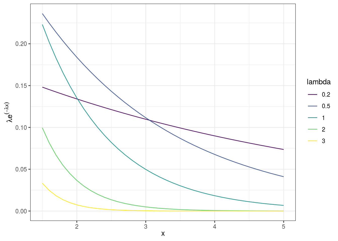
The likelihood is given by \(L(\lambda | x_1)=\lambda \exp^{- \lambda x_1}\).
Similarly, the likelihood of \(\lambda\) given our second measurement, \(x_2\) is given by \(L(\lambda | x_2) = \lambda \exp^{- \lambda x_2}\), and so on. It is the value of y (in y-axis) obtained by plugging in the value of \(x_1\) and \(x_2\) in the function.
So now, what is the likelihood of \(\lambda\) given both \(x_1\) and \(x_2\) ? We know individual likelihood functions as we present above. The combined likelihood function can be represented multiplication of two likelihood functions,
\[ \begin{align} L(\lambda | x_1 \text{ and } x_2) &= L(\lambda | x_1) L(\lambda | x_2) \\ &= \lambda \exp^{-\lambda x_1}.\lambda \exp^{-\lambda x_2} \\ &= \lambda^2[\exp^{-\lambda x_1}. \exp^{-\lambda x_2}] \\ &= \lambda^2[\exp^{-\lambda(x_1 + x_2)}] \end{align} \]
The the last equation is the likelihood of \(\lambda\) given \(x_1\) and \(x_2\).
What is the likelihood of \(\lambda\) given all of the data, \(x_1, x_2, x_3, \ldots, x_n\) ?
It is combined likelihood of observing all data values.
\[ \begin{align} L(\lambda | x_1, x_2, x_3, \ldots, x_n) &= L(\lambda | x_1) L(\lambda | x_2) L(\lambda | x_3) \ldots L(\lambda | x_n) \\ &= \lambda e^{-\lambda x_1}.\lambda e^{-\lambda x_2}.\lambda e^{-\lambda x_3} \\ &= \lambda^n[e^{-\lambda x_1}e^{-\lambda x_2}\ldots e^{-\lambda x_3}] \\ &= \lambda^n[e^{-\lambda(x_1 + x_2 + x_3 + \ldots + x_n)}] \end{align} (\#eq: likelihood-fun) \]
Now an issue could be, what if we don’t have a good value of \(\lambda\) ? One solution is we could try different values for \(\lambda\) to find a good one. To find the maximum likelihood,
- Take the derivative of likelihood-fun
- Solve for \(\lambda\) when the derivative is set to be equal to 0.
Now let us again consider the values of \(x_i\) (the time interval between two successive viewership of channes, in our previous example).
| x |
|---|
| 1.5 |
| 1.6 |
| 1.7 |
| 1.8 |
| 1.9 |
| 2.0 |
| 2.1 |
| 2.2 |
| 2.3 |
| 2.4 |
| 2.5 |
| 2.6 |
| 2.7 |
| 2.8 |
| 2.9 |
| 3.0 |
| 3.1 |
| 3.2 |
| 3.3 |
| 3.4 |
| 3.5 |
| 3.6 |
| 3.7 |
| 3.8 |
| 3.9 |
| 4.0 |
| 4.1 |
| 4.2 |
| 4.3 |
| 4.4 |
| 4.5 |
| 4.6 |
| 4.7 |
| 4.8 |
| 4.9 |
| 5.0 |
Now the relationship between likelihood values using different sets of \(\lambda\) can be seen as:
## `summarise()` ungrouping output (override with `.groups` argument)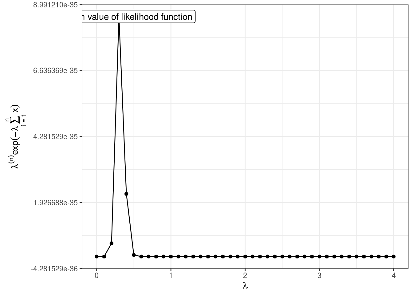
Noticeably, this function is ugly because of too small or too large estimated values. This function initially rises, but finally starts to slow down. This can be seen at the point when likelihood value starts to decrease – point of inflection. This point can also be obtained by setting the slope of likelihood function (derivative) to 0.
But before that we may take the log of the combined likelihood function. This is because the derivative of a function and the derivative of the log of a function equal 0 at the same place. So, for the purpose of finding where the derivative equals 0, the original function and its log are interchangeable. Thus we have the log of likelihood function is:
log likelihood function can be plotted against lambda looks,
## `summarise()` ungrouping output (override with `.groups` argument)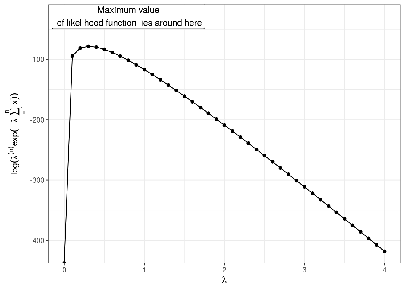
When we can specify the log form, multiplicative terms of initial function – \(\lambda\) and \(\exp\) can now be added as shown in derivative of log likelihood function with respect to \(\lambda\),
\[ \begin{align} \frac{\delta}{\delta \lambda} L(\lambda | x_1, x_2, x_3, \ldots, x_n) &= \frac{\delta}{\delta \lambda} \log (\lambda^n[\exp^{-\lambda(x_1 + x_2 + x_3 + \ldots + x_n)}]) \\ &= \frac{\delta}{\delta \lambda} \log (\lambda^n) + \log[\exp^{-\lambda(x_1 + x_2 + x_3 + \ldots + x_n)}]) \\ &= \frac{\delta}{\delta \lambda} n\log (\lambda) -\lambda(x_1 + x_2 + x_3 + \ldots + x_n) \end{align} \]
Finally taking the derivative, and setting the value to 0, we get:
\[ 0 = n \frac{1}{\lambda}-(x_1 + x_2 + x_3 + \ldots + x_n) \]
Solving for \(\lambda\) give,
\[ \lambda = \frac{n}{(x_1 + x_2 + x_3 + \ldots + x_n)} \]
Now, whenever we collect a lot of data about how much time takes place between events, we just plug those values into this equation and we’ll get the maximum likelihood estimate for \(\lambda\) and then we can fit an exponential distribution to our data.
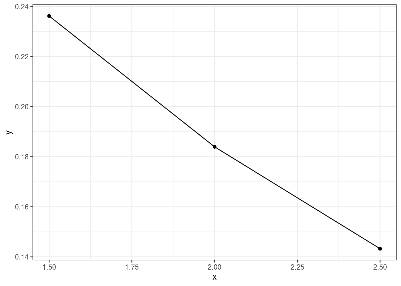
Hence, we can see that, for example, if 2 seconds passed between 1st and 2nd times a video was watched \((x_1 = 2)\), 2.5 seconds passed between 2nd and 3rd times the video was watched \((x_2 = 2.5)\) and 1.5 seconds passed between 3rd and 4th time the video was watched \((x_3 = 1.5)\), we can have the maximum likelihood estimate,
\[ \lambda = \frac{3}{2 + 2.5 + 1.5} = 0.5 \]
Thus, given the data, the maximum likelihood estimate for \(\lambda\) is 0.5. Graphically,
## geom_path: Each group consists of only one observation. Do you need to adjust
## the group aesthetic?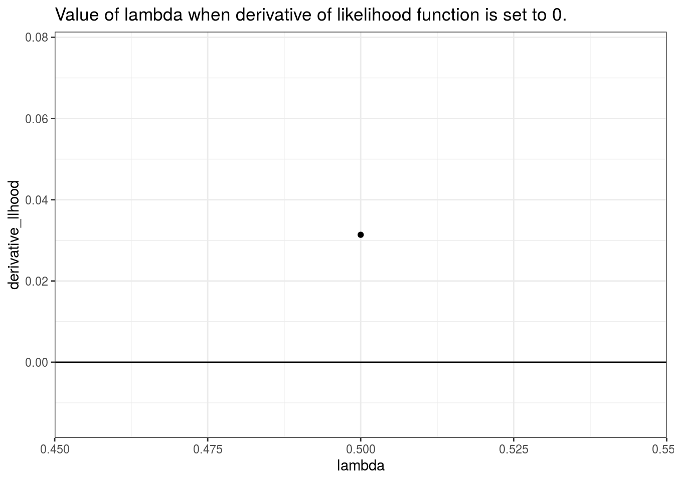
Inverse function and its distribution