Linear model fitting for regression: Basics and Variation

Linear model (simple forms) fitting

I use mtcars dataset to construct some basic regression models and fit those.

# convert available data to use in fitting
mtcars_reg_df <- mtcars %>% 
  rownames_to_column("carnames") %>% 
  as_tibble() %>% 
  mutate_at(c("gear", "am", "vs", "cyl"), as.factor)

We will be comparing difference between cylinder means for mpg.

# # intercept only lm tidiying and visualization
mpg_model1 <- mtcars_reg_df %>%
  group_by(cyl) %>%
  nest() %>%
  group_by(cyl) %>%
  mutate(mpg_model = map(data, ~lm(`mpg` ~ 1, .x))) %>%
  mutate(
    # rsqrd = map_dbl(mpg_model, ~summary(.x)[['r.squared']]), # this is '0' of intercept only model
    intercept_pvalue = map_dbl(mpg_model, ~summary(.x)[['coefficients']][1, 4]),
    intercept_se = map_dbl(mpg_model, ~summary(.x)[['coefficients']][1, 2]),
    intercept_coef = map_dbl(mpg_model, ~summary(.x)[['coefficients']][1, 1])
  ) %>%
  select(cyl, mpg_model, contains("intercept"), data)

Intercept-only models (each group fitted a different one) are plotted to reflect variation in estimated parameters. Two methods can be used to obtain same result. In the first, standard error obtained from model summary can be directly used; in the other SE can be manually computed.

# # method 1
mpg_model1 %>%
  select(-data, -contains("model")) %>%
  ggplot(aes(x = cyl, y = intercept_coef)) +
  geom_point() +
  geom_errorbar(aes(ymin = intercept_coef-intercept_se, ymax = intercept_coef+intercept_se)) +
  labs(x = "Number of cylinders",
       y = "MPG",
       title = "Mean MPG differs among cars with different cylinder numbers") +
  theme(text = element_text(size = 12), axis.text.x = element_text(angle = 30))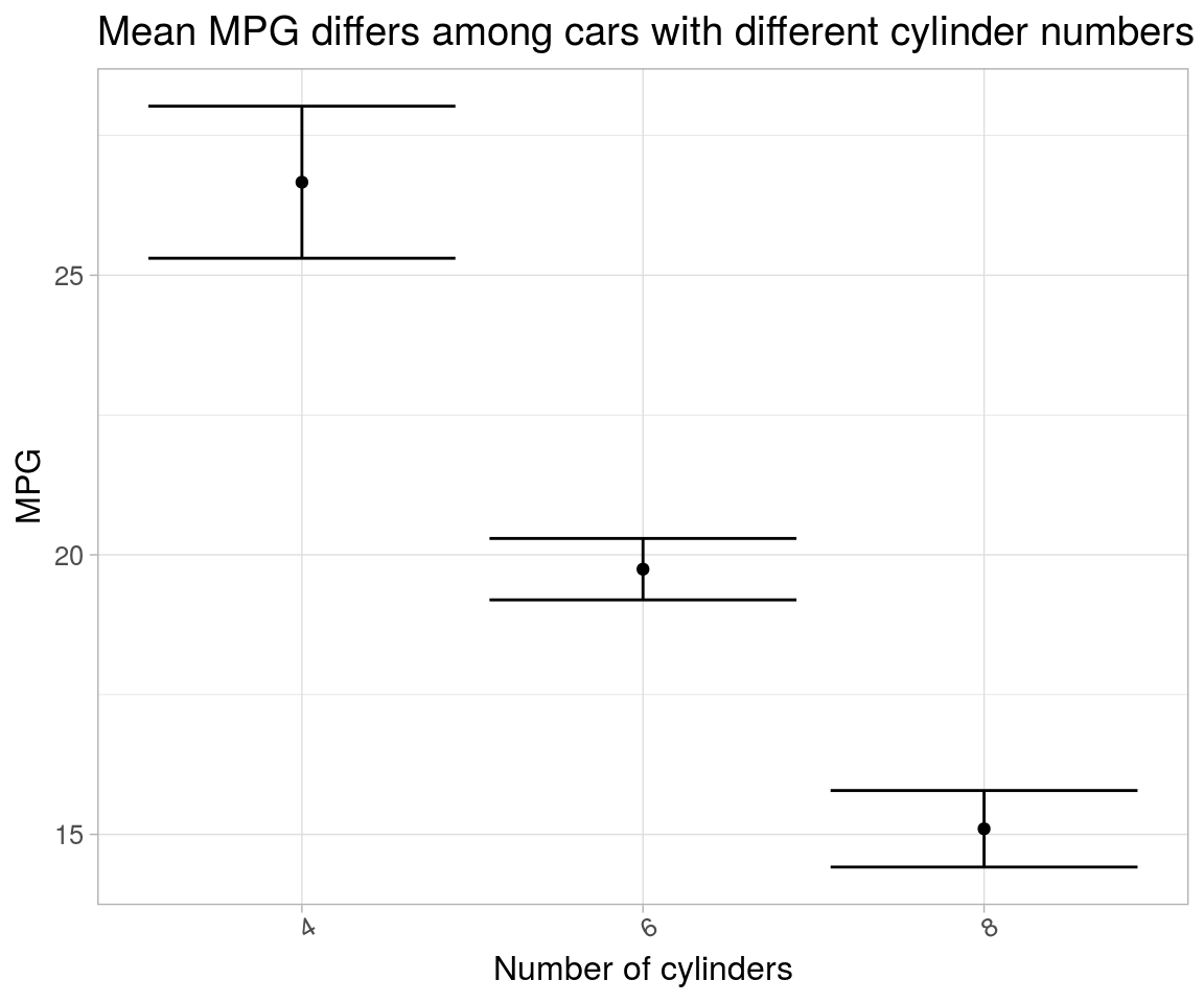

# # method 2
# same as method 1
mtcars_reg_df %>%
  group_by(cyl) %>%
  summarise_at("mpg", list(~mean(.), ~sd(.), ~n(),
                           q95 = ~quantile(., 0.95),
                           q75 = ~quantile(., 0.75),
                           q25 = ~quantile(., 0.25),
                           q5 = ~quantile(., 0.05))) %>%
  mutate(`se` = `sd`/sqrt(`n`)) %>%
  mutate(`left95` = `mean` - 2 * `se`,
         `right95` = `mean` + 2 * `se`) %>%
  ggplot(aes(x = `cyl`, y = `mean`)) +
  geom_point() +
  # # plot only errorbars with
  # geom_errorbar(aes(ymin = `left95`, ymax = `right95`)) +
  # or plot several quantiles with
  geom_crossbar(aes(ymin = `q5`, ymax = `q95`),
                fill = "aquamarine1",  color = "aquamarine1", width = 0.2) +
  geom_crossbar(aes(ymin = `q25`, ymax = `q75`),
                fill = "aquamarine4",  color = "aquamarine4", width = 0.2) +
  geom_crossbar(aes(ymin = `left95`, ymax = `right95`),
                fill = "black", color = "black", width = 0.2) +
  labs(x = "Number of cylinders",
       y = "MPG",
       title = "Mean MPG differs among cars with different cylinder numbers") +
  theme(text = element_text(size = 12), axis.text.x = element_text(angle = 30))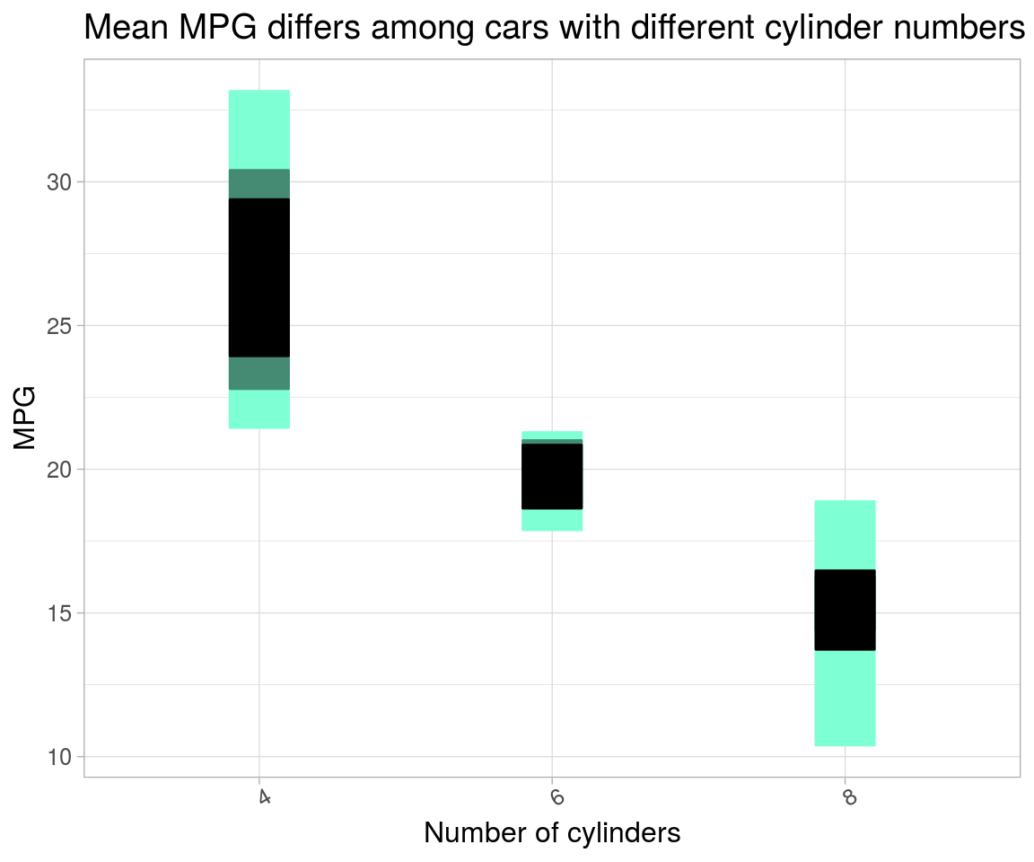

Showing intercept and slope model in the plot is less useful, as it has only two (different) standard error estimates – one for an intercept (dummy; ), and others for slopes () all intercept-coefficients. For e.g. the model,

lm(`mpg`~`cyl, data = mtcars_reg_df)

is less useful for comparing simple effects of factor means.

Yet another variation of linear model is constructing a slope only model using coefficients and their SEs for plotting.

# # method 3
lm(`mpg`~`cyl`-1, data = mtcars_reg_df) %>% 
  # summary() %>% coefficients() %>% 
  broom::tidy() %>%
  ggplot(aes(x = term, y = estimate)) +
  geom_point() +
  geom_errorbar(aes(ymin = estimate-std.error, ymax = estimate+std.error)) +
  labs(x = "Number of cylinders",
       y = "MPG",
       title = "Mean MPG differs among cars with different cylinder numbers") +
  theme(text = element_text(size = 12), axis.text.x = element_text(angle = 30))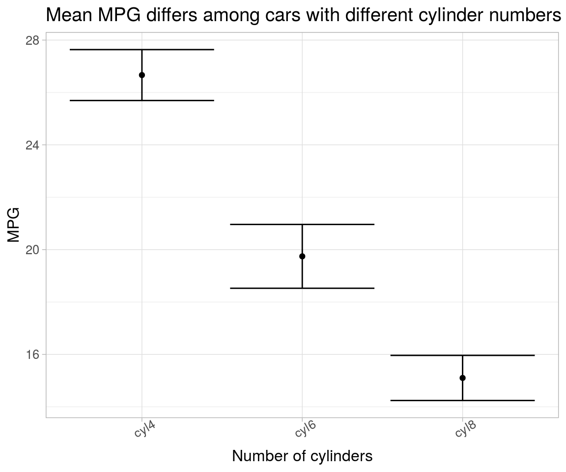

Note that, here, slope shows a different distribution than that of intercept distribution.