Layout and visualization of experimental design
Functional approach to creating and combing multiple plots
This approach highlights features of gridExtra package that allows combining multiple grob plots using function calls.
We explicitly use lapply/split or similar class of purrr functions to really scale the graphics.
We load a Hybrid maize trial dataset, with fieldbook generated using agricolae::design.rcbd(). The dataset looks as shown in Table 1, after type conversion and cleaning.
| Rep | Block | Plot | Entry | col | row | tillering | moisture1 | moisture2 | Ear count | Plant height |
|---|---|---|---|---|---|---|---|---|---|---|
| 1 | 1 | 1 | 1 | 1 | 1 | 3.0 | 3.5 | 35 | 270 | |
| 1 | 1 | 2 | 3 | 1 | 2 | 3.0 | 3.5 | 25 | 266 | |
| 1 | 1 | 3 | 18 | 1 | 3 | 3.5 | 4.0 | 30 | 261 | |
| 1 | 1 | 4 | 32 | 1 | 4 | 4.0 | 4.5 | 26 | 224 | |
| 1 | 1 | 5 | 37 | 1 | 5 | 4.0 | 4.5 | 30 | 268 | |
| 1 | 2 | 6 | 27 | 1 | 6 | 4.0 | 4.5 | 20 | 268 | |
| 1 | 2 | 7 | 21 | 1 | 7 | 4.0 | 4.5 | 25 | 277 | |
| 1 | 2 | 8 | 13 | 1 | 8 | 3.5 | 4.0 | 25 | 264 |
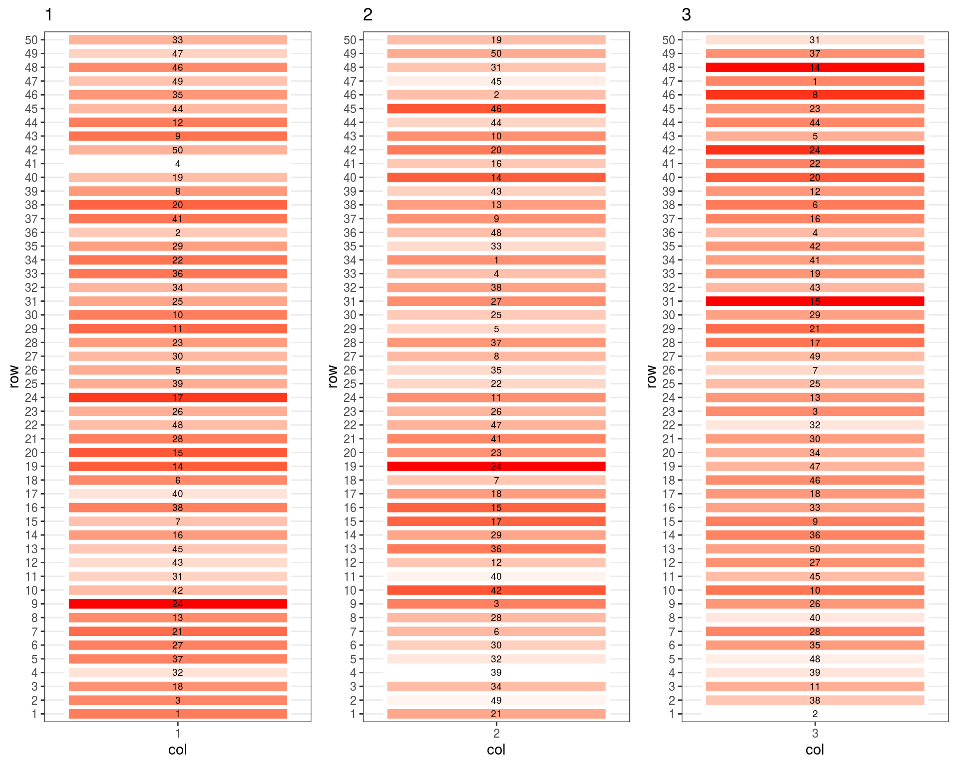
For the given dataset, we can draw on the information that Rep variable was used as field level blocking factor (Although separate, Block, variable exists, it was nested inside the Rep.) Therefore, to begin with, we ignore other spatial grouping variable. Now, since the grid graphics only requires two way represenation of plotting data, we have row and col information feeding for that.
Plotting call
Lattice graphics approach
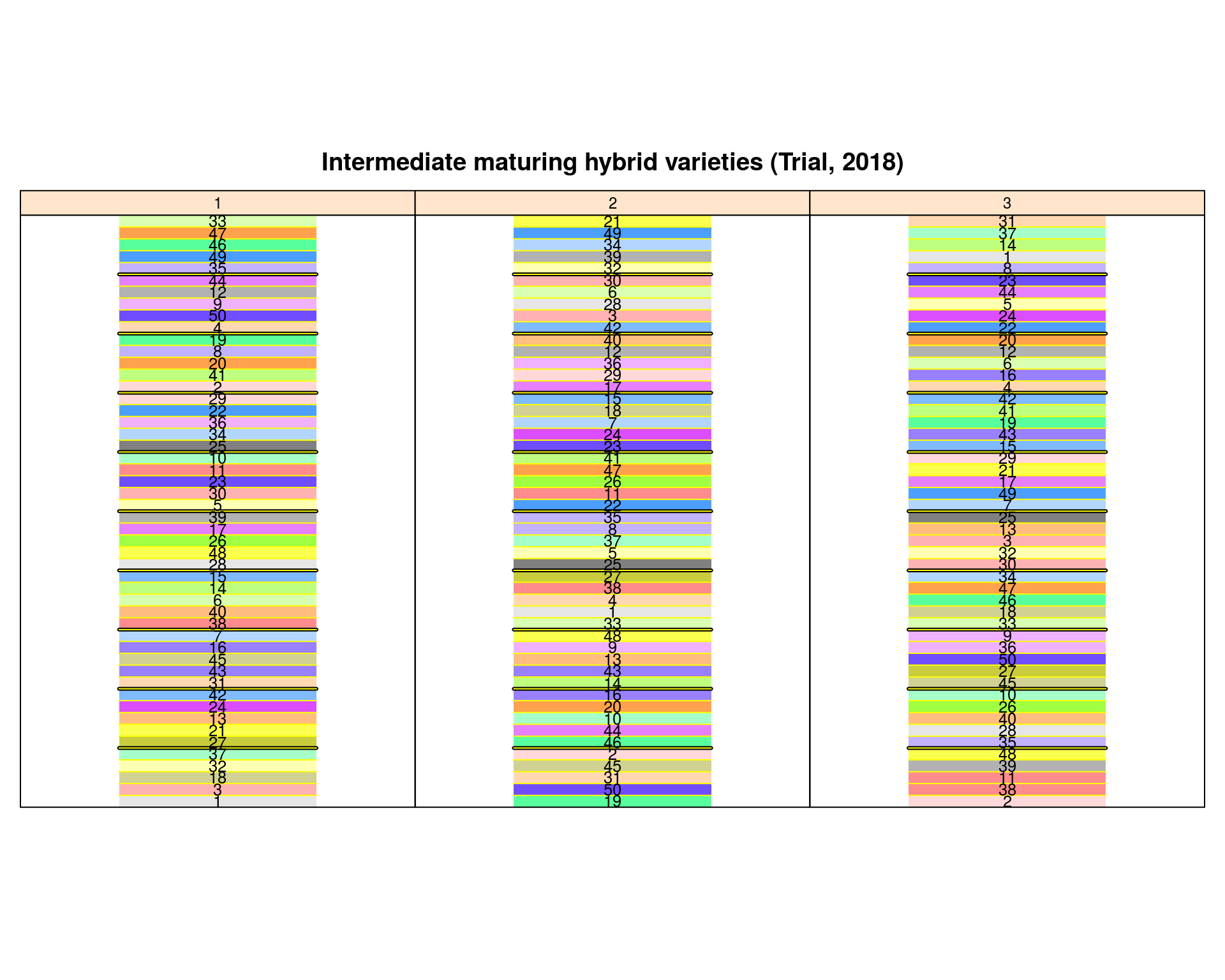
Using built-in function desplot() in desplot package, we can generate similar field design layout. In the plot below, individual entries (a factor variable) are highlighted as cell features. The process follows as shown below. In addition to default plotting, we can also generate serpentine design layout using simple mutating trick. Plus, block grouping has also been added to show the nested factor component.
Note: In order to plot in required layout, just specify: layout = c(number_of_rows, number_of_columns) argument (Thanks to Kevin Wright for helping me figure this out.)