Design and analysis of balanced randomized complete block (RCBD) experiment
Introduction
Balanced block designs are a class of randomized experimental design that contain equal number of records for a particular level of categorical variable across all blocks.
Example 1
Let us generate some data from random process mimicking a single factor process consisting of 3 levels.
A glimpse of what data looks like is shown in Table 1.
| Treatment | Block | Value |
|---|---|---|
| Treatment1 | a | -0.629 |
| Treatment2 | a | -2.565 |
| Treatment3 | a | -1.637 |
| Treatment4 | a | -1.367 |
| Treatment5 | a | -1.596 |
| Treatment6 | a | -2.106 |
| Treatment7 | a | -0.488 |
| Treatment8 | a | -2.095 |
The agricolae::design.rcbd() function generates design and the field book associated with the design. The field book looks like the one below in Table 2
| plots | block | treatments |
|---|---|---|
| 101 | 1 | Treatment28 |
| 102 | 1 | Treatment5 |
| 103 | 1 | Treatment27 |
| 104 | 1 | Treatment24 |
| 105 | 1 | Treatment9 |
| 106 | 1 | Treatment16 |
| 107 | 1 | Treatment3 |
| 108 | 1 | Treatment30 |
Box Plots
To deal with real case scenario, let’s import a dataset from hybrid maize trial of intermediate duration maturing types, which was conducted on summer of 2018. The plant height trait will be dealt.
After import, type conversion and cleaning the data looks like as shown in Table 3
| Rep | Block | Plot | Entry | col | row | tillering | moisture1 | moisture2 | Ear count | Plant height |
|---|---|---|---|---|---|---|---|---|---|---|
| 1 | 1 | 1 | 1 | 1 | 1 | 3.0 | 3.5 | 35 | 270 | |
| 1 | 1 | 2 | 3 | 1 | 2 | 3.0 | 3.5 | 25 | 266 | |
| 1 | 1 | 3 | 18 | 1 | 3 | 3.5 | 4.0 | 30 | 261 | |
| 1 | 1 | 4 | 32 | 1 | 4 | 4.0 | 4.5 | 26 | 224 | |
| 1 | 1 | 5 | 37 | 1 | 5 | 4.0 | 4.5 | 30 | 268 | |
| 1 | 2 | 6 | 27 | 1 | 6 | 4.0 | 4.5 | 20 | 268 | |
| 1 | 2 | 7 | 21 | 1 | 7 | 4.0 | 4.5 | 25 | 277 | |
| 1 | 2 | 8 | 13 | 1 | 8 | 3.5 | 4.0 | 25 | 264 |
Although the block component exists for given dataset, for the sake of making case with analysing single factor RCBD experiment, we ignore the factor the effect.
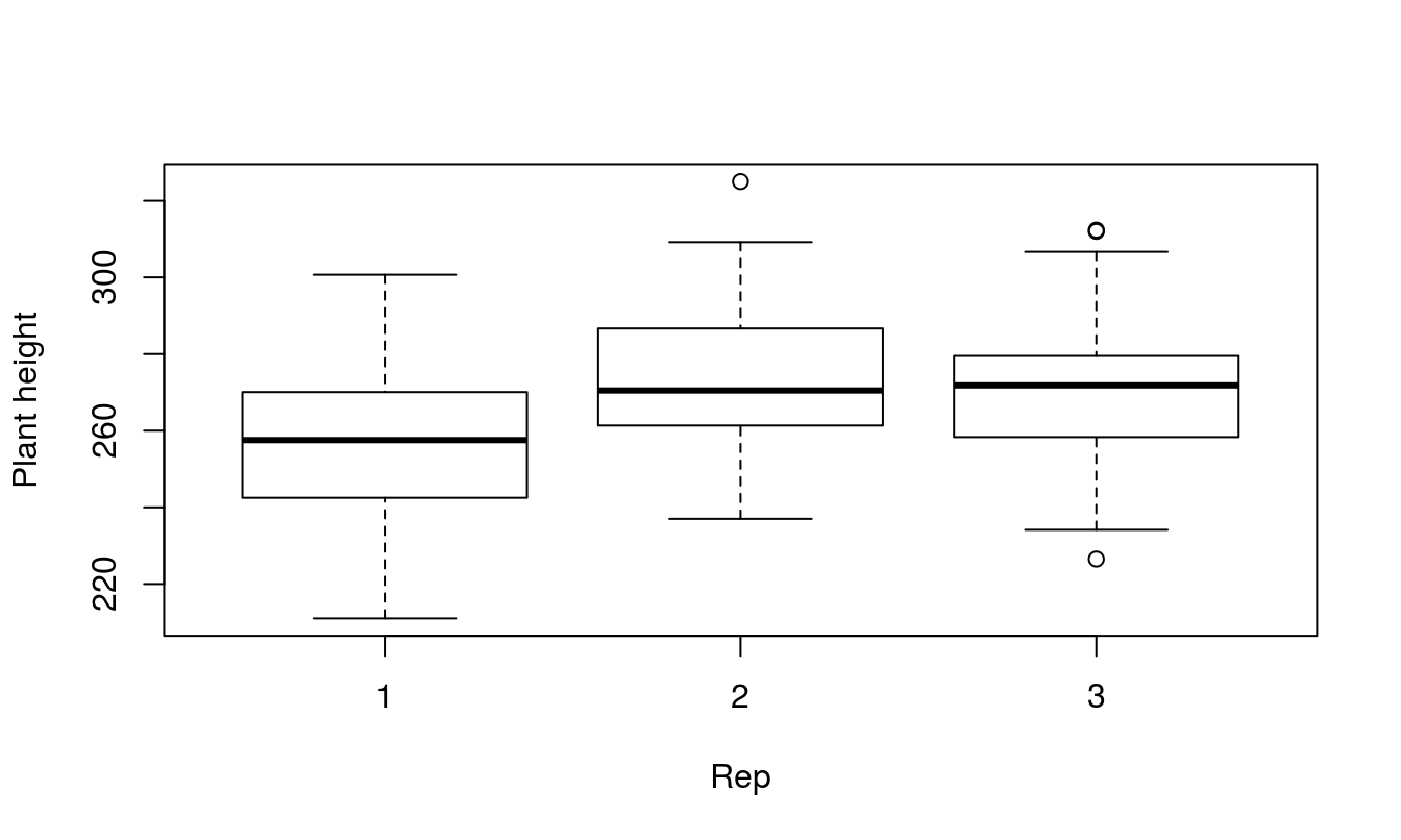
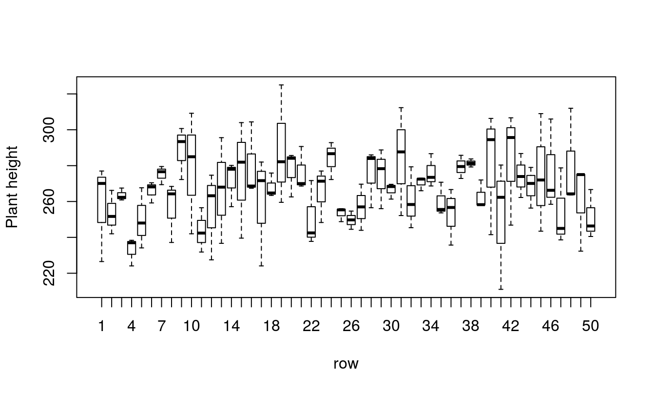
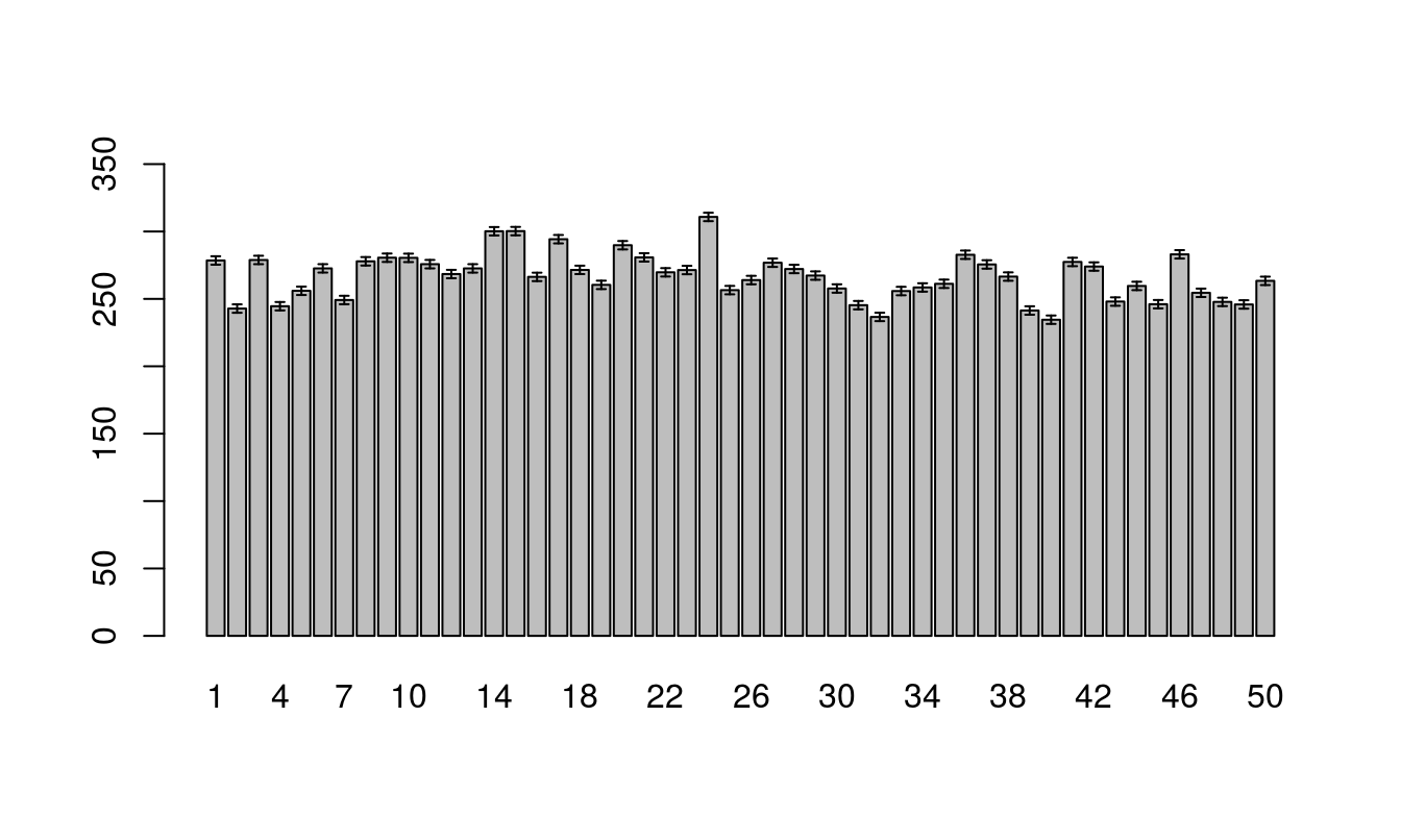
A good thing to start with is plots of the data. Box plots are good for checking constant variances and to look for outliers.
Balanced?
It is always a good idea to check to see if the data is balanced.
table(ihyb_multiple$Entry)##
## 1 2 3 4 5 6 7 8 9 10 11 12 13 14 15 16 17 18 19 20 21 22 23 24 25 26
## 3 3 3 3 3 3 3 3 3 3 3 3 3 3 3 3 3 3 3 3 3 3 3 3 3 3
## 27 28 29 30 31 32 33 34 35 36 37 38 39 40 41 42 43 44 45 46 47 48 49 50
## 3 3 3 3 3 3 3 3 3 3 3 3 3 3 3 3 3 3 3 3 3 3 3 3# with(ihyb_multiple, table(Entry, Rep)) # if two
# way table is to be generatedMeans
The means for each factor level can be calculated, as well as for combination of different factor levels. The notation for the an interaction is “A:B”.
##   1   2   3   4   5   6   7   8   9  10  11  12  13  14  15  16  17  18  19  20
## 278 243 279 245 256 273 249 278 281 280 276 268 273 300 300 266 294 272 260 290
##  21  22  23  24  25  26  27  28  29  30  31  32  33  34  35  36  37  38  39  40
## 281 270 271 311 256 264 277 272 267 258 245 237 256 258 261 283 276 267 241 235
##  41  42  43  44  45  46  47  48  49  50
## 277 274 248 260 246 283 255 248 246 263
## 1 2 3
## 257 274 270Treatment Mean Plots/Interaction Plots
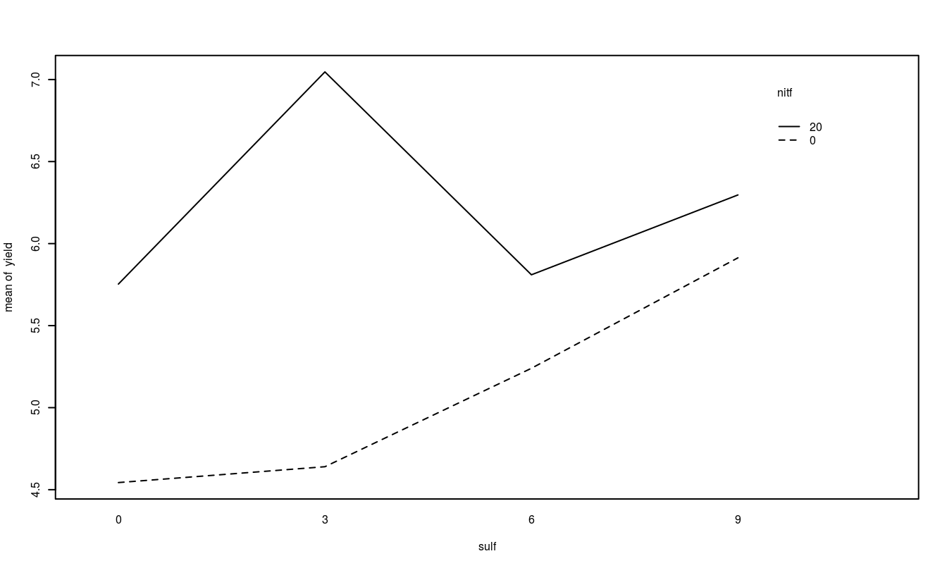
The other plot that is useful is the treatment means plot. It is a good idea to look at it both ways and look for possible interactions.

Running the ANOVA
After the priliminary diagnostics is done, and transformations are made (if required), next we model the variable relationships.
There are two ways to conduct the variance analysis in R – one specifying a regression model, the other by speficying a variance component model. Since, we are dealing with single factor experiment with replicates, we can use model formula \(A+B\) for specifying the regressors or a.k.a grouping variables (in case of factorial ANOVA), where \(A\) is the factor of interest and \(B\) is the recogizable source of source variation controlled through replication/blocking. The standard model for a randomized complete block design (with \(s = 1\) observation on each treatment in each block) is
\[ Y_{hi} = \mu + \theta_h + \tau_i + \epsilon_{hi}, \\ \epsilon_{hi}\sim N(0, \sigma^2), \\ {\epsilon_{hi}}'s\ are\ mutually\ independent, \\ h = 1,..., b;\ i = 1,..., v , \]
Where \(\mu\) is a constant, \(\theta_h\) is the effect of the \(h_{th}\) block, \(\tau_i\) is the effect of \(i_{th}\) treatment, \(Y_{hi}\) is the random variable representing the measurement on treatment \(i\) observed on block \(j\), and \(\epsilon_{hi}\) is the random error associated. This form of standard model is called block-treatment model.
This model is limiting in that it does not include a term for interaction between blocks and treatments. However, including the interaction term in the model will lead to absence of degrees of freedom for estimation of error variance. It is also imperative to assume, in several blocking experiments, that interaction is non significant. There appears to be a case where interaction component could be estimated: when block size is increased during the design. For further explaination refer to Dean, Voss, and Draguljić (2017).
The block-treatment model is similar to two-way main-effects model for two treatment factors in a completely randomized design with one observation per cell. The only difference between CRD and RCBD here is that in former experimental units are randomly assigned to treatment combinations (and, therefore to the levels of both factors) while in RCBD, the experimental units are randomly assigned to the levels of the treatment factor only. The levels of the block factor represent intentional groupings of the experimental units.
The standard block-treatment model implementation of RCB design using Plant height as response variable is coded below. The model ANOVA is shown in Table 4. We first plot the residuals and the Box-Cox plot to check assumptions. Once we are satisfied, we can examine the ANOVA.
res <- aov(`Plant height` ~ Rep + Entry, data = ihyb_multiple)
plot(res, 1)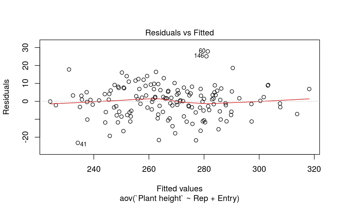
# # test for homogeneity of variance
# bartlett.test(`Plant
# height`~Rep,data=ihyb_multiple)
# bartlett.test(`Plant
# height`~Entry,data=ihyb_multiple)
# boxcox diagnostics
boxCox(res) # if lambda parameter lies near to zero then, log transformation is useful to maintain assumption about distribution of the variable for further tests.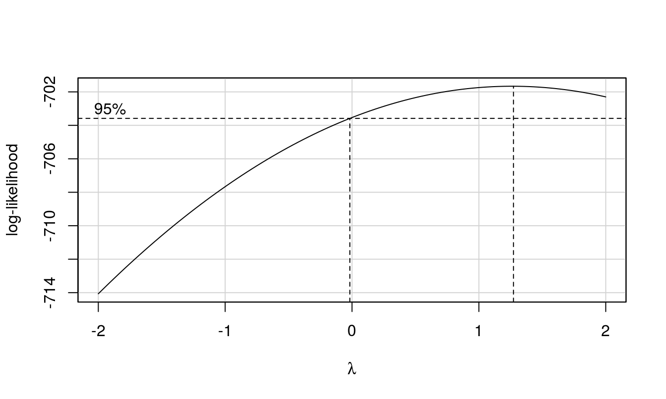
The residuals look good and the Box-Cox plot indicates no transformation is needed.
| Df | Sum Sq | Mean Sq | F value | Pr(>F) | |
|---|---|---|---|---|---|
| Rep | 2 | 8534 | 4267 | 36.13 | 0 |
| Entry | 49 | 42993 | 877 | 7.43 | 0 |
| Residuals | 98 | 11575 | 118 |
Means and Tukey HSD
R has some additional commands to find means as well as the effects of each factor level (think \(\alpha_i\) and \(\beta_i\)). Since both the replication and the entry effects are significant, we require Tukey pairwise comparisons test to distinguish which two among the levels of each factors are different.
model.tables(res, "means")## Tables of means
## Grand mean
##
## 267
##
## Rep
## Rep
##   1   2   3
## 257 274 270
##
## Entry
## Entry
## 1 2 3 4 5 6 7 8 9 10 11 12 13 14 15 16 17 18 19 20
## 278 243 279 245 256 273 249 278 281 280 276 268 273 300 300 266 294 272 260 290
## 21 22 23 24 25 26 27 28 29 30 31 32 33 34 35 36 37 38 39 40
## 281 270 271 311 256 264 277 272 267 258 245 237 256 258 261 283 276 267 241 235
## 41 42 43 44 45 46 47 48 49 50
## 277 274 248 260 246 283 255 248 246 263model.tables(res, "effects")## Tables of effects
##
## Rep
## Rep
## 1 2 3
## -10.36 7.38 2.99
##
## Entry
## Entry
## 1 2 3 4 5 6 7 8 9 10 11
## 11.58 -24.09 11.95 -22.35 -10.92 5.71 -17.76 10.96 13.62 13.51 8.85
## 12 13 14 15 16 17 18 19 20 21 22
## 1.51 5.70 33.25 33.36 -0.60 27.36 4.59 -6.52 22.89 13.87 2.79
## 23 24 25 26 27 28 29 30 31 32 33
## 4.48 43.87 -10.42 -2.96 9.91 5.26 0.38 -9.21 -21.58 -30.30 -11.11
## 34 35 36 37 38 39 40 41 42 43 44
## -8.43 -5.73 15.82 8.63 -0.37 -25.54 -32.37 10.48 7.07 -18.90 -7.32
## 45 46 47 48 49 50
## -20.85 16.13 -12.41 -19.16 -21.05 -3.55# tukey honestly significant difference
TukeyHSD(res, "Entry")$Entry %>% head()## diff lwr upr p adj
## 2-1 -35.67 -72.3 0.952 0.0691
## 3-1 0.37 -36.3 36.996 1.0000
## 4-1 -33.93 -70.6 2.693 0.1200
## 5-1 -22.50 -59.1 14.127 0.9159
## 6-1 -5.86 -42.5 30.762 1.0000
## 7-1 -29.34 -66.0 7.289 0.3913Since there are significant differences between the entries, a plot of the means may be appropriate. We can use the model.tables() to obtain the means (it behaves similar to tapply()).
Example 2
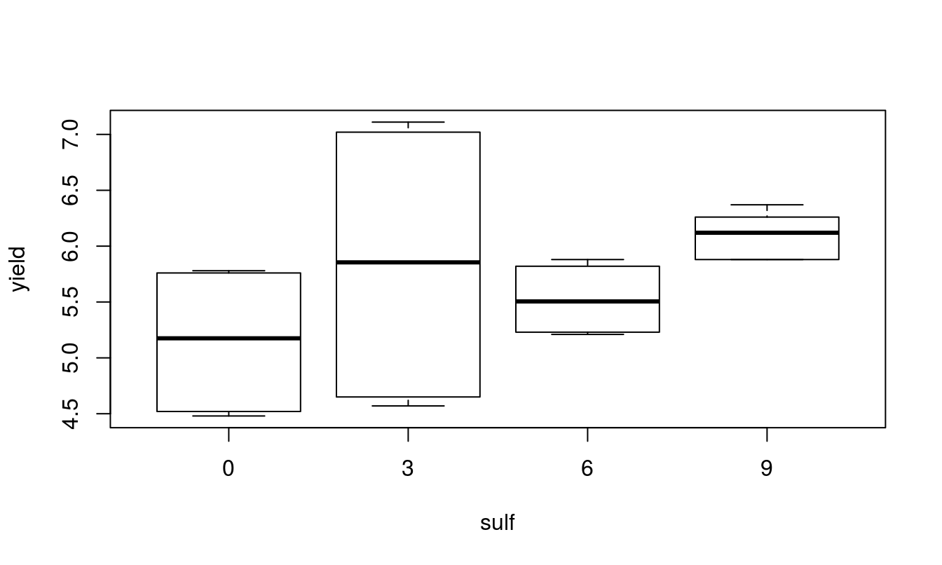
In this example, we wish to see how the addition of sulphur and nitrogen affect the yield (bushels per acre) of soybeans(data source: “http://personal.psu.edu/~mar36/stat_461/sulpher.csv”). The final goal is to determine which combination, if any, of sulphur and nitrogen produces the highest yield.
## # A tibble: 6 x 3
##   nitrogen sulpher yield
##      <dbl>   <dbl> <dbl>
## 1        0       0  4.48
## 2        0       0  4.52
## 3        0       0  4.63
## 4        0       3  4.7
## 5        0       3  4.65
## 6        0       3  4.57
## # A tibble: 6 x 5
## nitrogen sulpher yield sulf nitf
## <dbl> <dbl> <dbl> <fct> <fct>
## 1 0 0 4.48 0 0
## 2 0 0 4.52 0 0
## 3 0 0 4.63 0 0
## 4 0 3 4.7 3 0
## 5 0 3 4.65 3 0
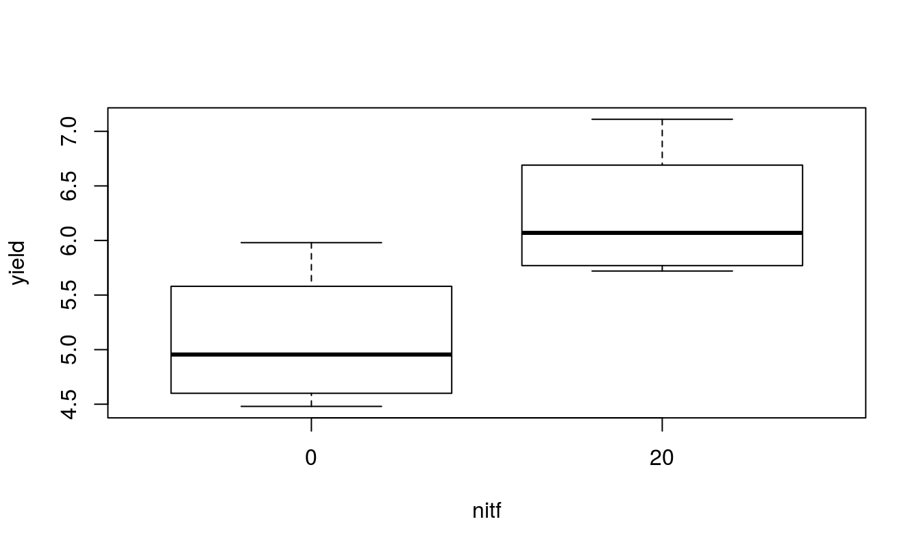
## 6 0 3 4.57 3 0A quick look at the data and a check to see if it is balanced. Do the treatment means plots indicate a significant interaction?
##     nitf
## sulf 0 20
##    0 3  3
##    3 3  3
##    6 3  3
##    9 3  3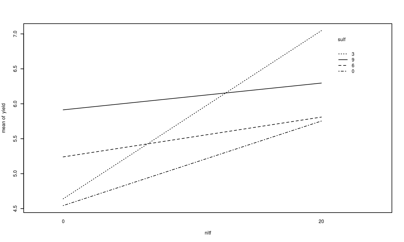
Residuals and Box-Cox plot
res.2 <- aov(yield ~ sulf * nitf, data = ex.2)
plot(res.2, 1)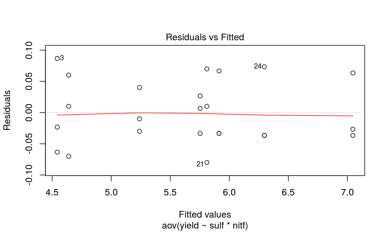
boxCox(res.2)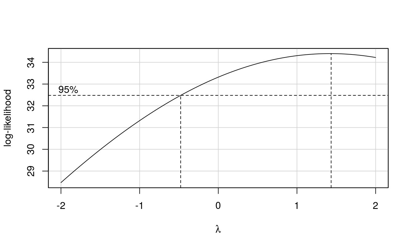
There seems to be no issues with the assumptions of ANOVA, so we will proceed to interpreting the results.
| term | df | sumsq | meansq | statistic | p.value |
|---|---|---|---|---|---|
| sulf | 3 | 3.069 | 1.023 | 286 | 0 |
| nitf | 1 | 7.832 | 7.832 | 2186 | 0 |
| sulf:nitf | 3 | 3.760 | 1.253 | 350 | 0 |
| Residuals | 16 | 0.057 | 0.004 |
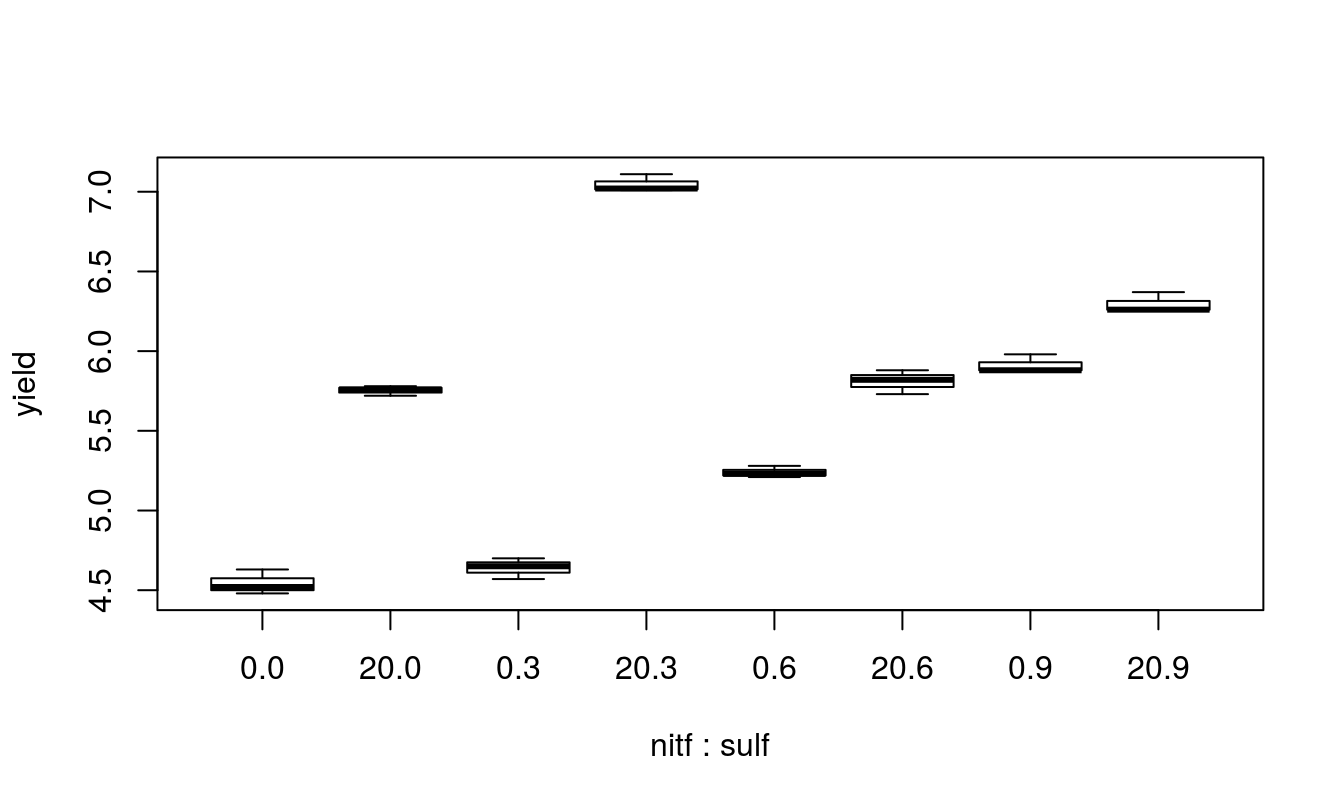
Based on the two-factor ANOVA analysis of soybean yield, there appears to be an interaction between the use of sulpher and nitrogen (F=349.78, num df=3, dem df=16, p-value=0). Since the interaction is significant, discussing the main effects individual is not possible, even though they themselves are significant (both p-values < 0.001). Applying nitrogen does increase yield but the amount of increase depends on the amount of sulpher used.
Since the interaction is significant, a good way to comprehend results is via a bar graph with grouping letters.
## [1] "sulf" "nitf" "sulf:nitf"## 3 6 9 0
## "a" "b" "c" "d"## 3:0 6:0 9:0 0:20 3:20 6:20 9:20 0:0
## "a" "b" "c" "c" "d" "c" "e" "a"## 0:0 0:20 3:0 3:20 6:0 6:20 9:0 9:20
## 4.54 5.75 4.64 7.05 5.24 5.81 5.91 6.30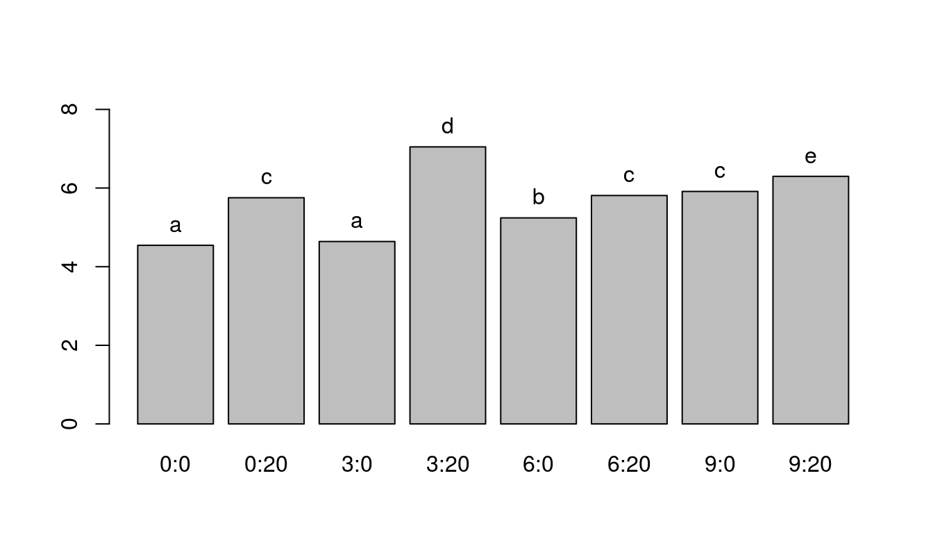
From the above plot, it appears that a combination of 3 units of sulpher and 20 units of nitrogen produce the highest yield of soybeans.
References
Dean, Angela, Daniel Voss, and Danel Draguljić. 2017. “Complete Block Designs.” In Design and Analysis of Experiments, 305–47. Springer.