Correlation and pathway analysis with path diagrams
Background
Correlation study is one of the most extensively yet not fully appreciated topic. It forms the backbone of several other inferential studies. Path analysis, on a similar note, is a derived technique that explains directed dependencies among a set of variables. It is almost exactly a century old now and still finds uses in several fields of causal inference.
In oder to understand the process of causal inference (thought to be successor of path analysis), it is important to understand the basics about categories of variables. Below I have pointed out some of the concepts.
Exogenous variable: Fully independent variable. Has only single arrow exitting from them. No single-headed arrows point at exogenous variables.
Endogenous variable: Variables that are solely dependent variables, or are both independent and dependent variables, are termed ‘endogenous’. Graphically, endogenous variables have at least one single-headed arrow pointing at them.
The Figure 1, two exogenous variables (Exogenous1 and Exogenous2) are modeled as being correlated as depicted by the double-headed arrow. Both of these variables have direct and indirect (through Endogenous2) effects on Endogenous1 (the two dependent or ‘endogenous’ variables/factors). In most real-world models, the endogenous variables may also be affected by variables and factors stemming from outside the model (external effects including measurement error). These effects are depicted by the “Influencer a” and “Influencer b” (error) terms in the model.
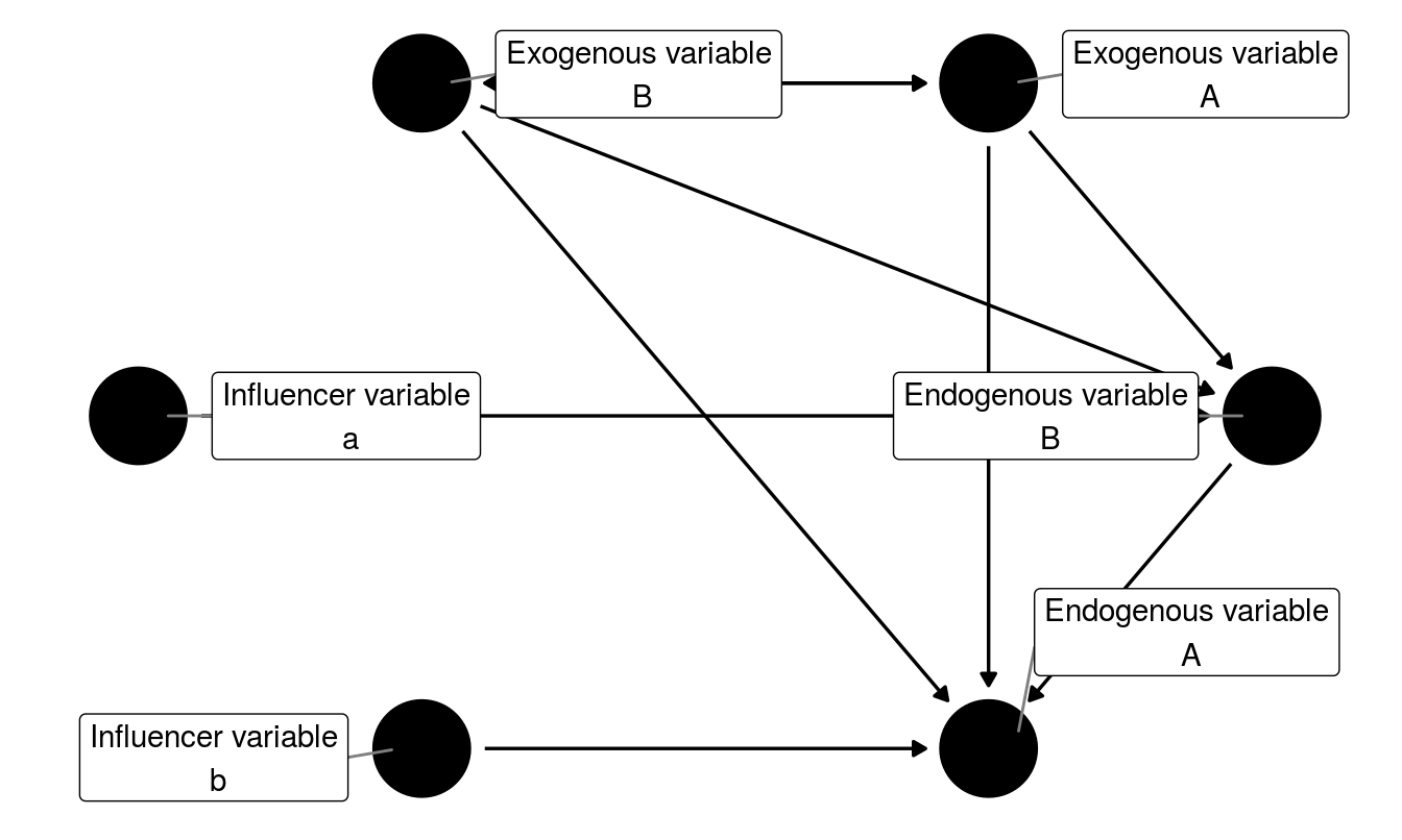
Figure 1: Variable types and modeling of relationship among them
This is one formulation of the several conceivable models, an alternative could assume that endogenous variable Endogenous2 has no role in relating Exogenous1 to Endogenous1 (No indirect effects). This could be represented as shown in Figure 2. Now the fit/likelihood of these these two models could be tested statistically.
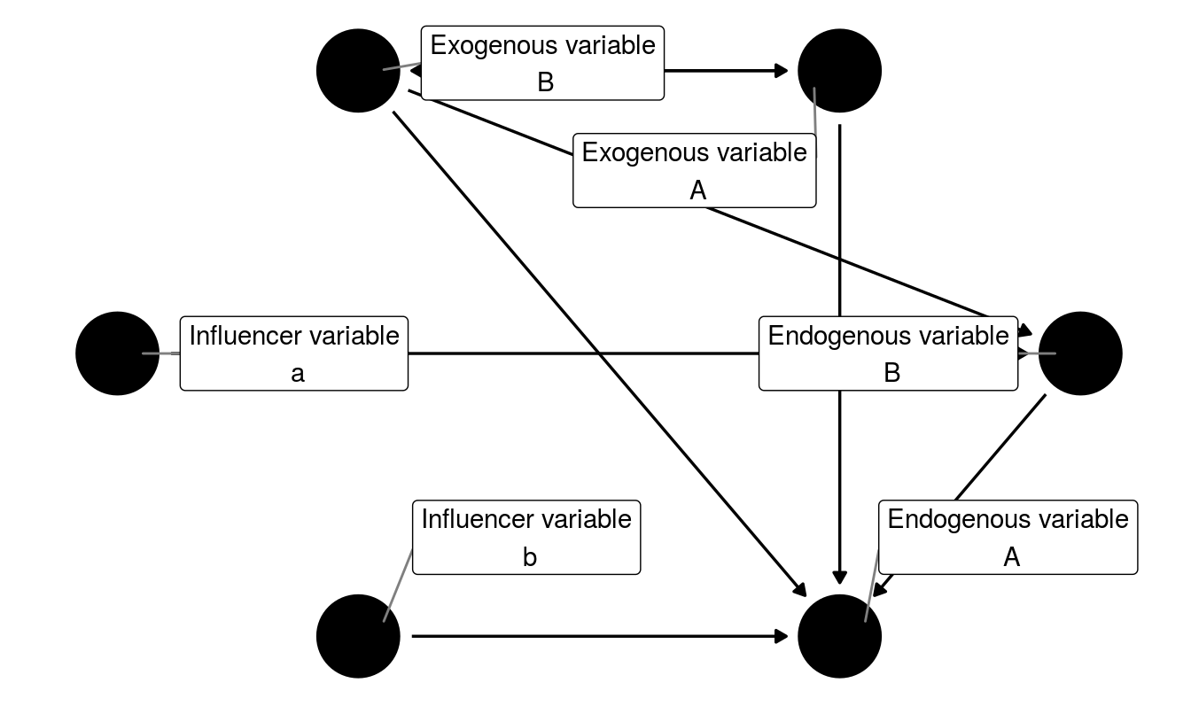
Figure 2: Variable types and modeling of relationship among them (alternative model)
Correlation analysis
After correlation matrix has been obtained, it is ready to be imported as is for analysis. Here, for example sake, an arbitrary correlation matrix has been used. To simulate a more messy and realistic scenario, we will use encoded correlation sheet where values are augmented with significance stars. The dataset looks is shown in Table 1.
| Variable | V1 | V2 | V3 | V4 | V5 | V6 | V7 | V8 | V9 | V10 |
|---|---|---|---|---|---|---|---|---|---|---|
| V1 | 1 | |||||||||
| V2 | -0.516* | 1 | ||||||||
| V3 | 0.983** | -0.516* | 1 | |||||||
| V4 | -0.398 | -0.02 | -0.44 | 1 | ||||||
| V5 | 0.794** | -0.086 | 0.812** | -0.530* | 1 | |||||
| V6 | 0.923** | -0.377 | 0.918** | -0.486 | 0.825** | 1 | ||||
| V7 | 0.853** | -0.458 | 0.854** | -0.548* | 0.817** | 0.819** | 1 | |||
| V8 | 0.674** | -0.573* | 0.638* | -0.222 | 0.388 | 0.547* | 0.815** | 1 | ||
| V9 | 0.669** | -0.549* | 0.638* | -0.334 | 0.442 | 0.567* | 0.863** | 0.976** | 1 | |
| V10 | 0.763** | -0.547* | 0.760** | -0.5 | 0.616* | 0.697** | 0.955** | 0.926** | 0.960** | 1 |
Path analysis
Detailed process of getting data ready for computing path coefficients is shown serially in code below. After completing the cleaning process, two matrix objects, one of dependent (corr_maty) and the other with explainatory variables (corr_matx) is required to pass to agricolae function path.analysis().
Now the prepared matrix objects look like what is shown in Tables 2 and 3.
| V1 | V2 | V4 | V5 | V6 | V7 | V8 | V9 | V10 | |
|---|---|---|---|---|---|---|---|---|---|
| V1 | 1.000 | -0.516 | -0.398 | 0.794 | 0.923 | 0.853 | 0.674 | 0.669 | 0.763 |
| V2 | -0.516 | 1.000 | -0.020 | -0.086 | -0.377 | -0.458 | -0.573 | -0.549 | -0.547 |
| V4 | -0.398 | -0.020 | 1.000 | -0.530 | -0.486 | -0.548 | -0.222 | -0.334 | -0.500 |
| V5 | 0.794 | -0.086 | -0.530 | 1.000 | 0.825 | 0.817 | 0.388 | 0.442 | 0.616 |
| V6 | 0.923 | -0.377 | -0.486 | 0.825 | 1.000 | 0.819 | 0.547 | 0.567 | 0.697 |
| V7 | 0.853 | -0.458 | -0.548 | 0.817 | 0.819 | 1.000 | 0.815 | 0.863 | 0.955 |
| V8 | 0.674 | -0.573 | -0.222 | 0.388 | 0.547 | 0.815 | 1.000 | 0.976 | 0.926 |
| V9 | 0.669 | -0.549 | -0.334 | 0.442 | 0.567 | 0.863 | 0.976 | 1.000 | 0.960 |
| V10 | 0.763 | -0.547 | -0.500 | 0.616 | 0.697 | 0.955 | 0.926 | 0.960 | 1.000 |
| V3 | |
|---|---|
| V1 | 0.983 |
| V2 | -0.516 |
| V4 | -0.440 |
| V5 | 0.812 |
| V6 | 0.918 |
| V7 | 0.854 |
| V8 | 0.638 |
| V9 | 0.638 |
| V10 | 0.760 |
We could check to see if dimensions of the matrix match, which is necessary for the calculation.
dim(corr_matx)## [1] 9 9dim(corr_maty)## [1] 9 1# Using agricolae function
path_coeffs <- agricolae::path.analysis(corr_matx,
corr_maty)$Coeff## Direct(Diagonal) and indirect effect path coefficients
## ======================================================
## V1 V2 V4 V5 V6 V7 V8 V9 V10
## V1 0.856 0.0619 -0.02896 0.6345 0.0449 -1.809 -0.2189 -0.1043 1.55
## V2 -0.442 -0.1199 -0.00146 -0.0687 -0.0183 0.971 0.1861 0.0856 -1.11
## V4 -0.341 0.0024 0.07276 -0.4235 -0.0236 1.162 0.0721 0.0521 -1.01
## V5 0.680 0.0103 -0.03856 0.7991 0.0401 -1.732 -0.1260 -0.0689 1.25
## V6 0.790 0.0452 -0.03536 0.6593 0.0486 -1.737 -0.1776 -0.0884 1.41
## V7 0.730 0.0549 -0.03987 0.6529 0.0398 -2.120 -0.2646 -0.1346 1.94
## V8 0.577 0.0687 -0.01615 0.3101 0.0266 -1.728 -0.3247 -0.1522 1.88
## V9 0.573 0.0658 -0.02430 0.3532 0.0276 -1.830 -0.3169 -0.1559 1.95
## V10 0.653 0.0656 -0.03638 0.4923 0.0339 -2.025 -0.3007 -0.1497 2.03
##
## Residual Effect^2 = 0.0121# path_coeffsIn fact, the path coefficients is just the result of matrix product between inverse matrix, of explainatory variables, and the dependent variable. For any Well-posed problem being modeled as ordinary least squares problem let us consider known vector \(A\) and \(b\). Now, we seek to find vector \(\mathbf{x}\). This could be solved as shown in the Equation (1).
\[\begin{equation} \tag{1} {\displaystyle A\mathbf {x} =\mathbf {b}} \\ {\displaystyle \mathbf{x} =A^{-1}\mathbf {b}} \end{equation}\]
Hence the solution for vector \(\mathbf x\) gives the direct effects path coefficients, between two variables. Then the indirect coefficients (\(Z\)) are scalar products of direct effects (\(\mathbf {x}\)) and correlation matrix of explainatory variables (\(A\)).
\[ Z = \mathbf {x} . A \]